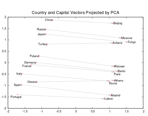
What’s useful about embeddings? Depending on who you ask, answers may vary. For many, the most immediate association may be word vectors and their use in natural language processing (translation, summarization, question answering etc.) There, they are famous for modeling semantic and syntactic relationships, as exemplified by this diagram found in one of the most influential papers on word vectors(Mikolov et al. 2013):
Others will probably bring up entity embeddings, the magic tool that helped win the Rossmann competition(Guo and Berkhahn 2016) and was greatly popularized by fast.ai’s deep learning course. Here, the idea is to make use of data that is not normally helpful in prediction, like high-dimensional categorical variables.
Another (related) idea, also widely spread by fast.ai and explained in this blog, is to apply embeddings to collaborative filtering. This basically builds up entity embeddings of users and items based on the criterion how well these “match” (as indicated by existing ratings).
So what are embeddings good for? The way we see it, embeddings are what you make of them. The goal in this post is to provide examples of how to use embeddings to uncover relationships and improve prediction. The examples are just that - examples, chosen to demonstrate a method. The most interesting thing really will be what you make of these methods in your area of work or interest.
Embeddings for fun (picturing relationships)
Our first example will stress the “fun” part, but also show how to technically deal with categorical variables in a dataset.
We’ll take this year’s StackOverflow developer survey as a basis and pick a few categorical variables that seem interesting - stuff like “what do people value in a job” and of course, what languages and OSes do people use. Don’t take this too seriously, it’s meant to be fun and demonstrate a method, that’s all.1
Preparing the data
Equipped with the libraries we’ll need:
We load the data and zoom in on a few categorical variables. Two of them we intend to use as targets: EthicsChoice and JobSatisfaction. EthicsChoice is one of four ethics-related questions and goes
“Imagine that you were asked to write code for a purpose or product that you consider extremely unethical. Do you write the code anyway?”
With questions like this, it’s never clear what portion of a response should be attributed to social desirability - this question seemed like the least prone to that, which is why we chose it.2
data <- read_csv("survey_results_public.csv")

data <- data %>% select(
  FormalEducation,
  UndergradMajor,
  starts_with("AssessJob"),
  EthicsChoice,
  LanguageWorkedWith,
  OperatingSystem,
  EthicsChoice,
  JobSatisfaction
)

data <- data %>% mutate_if(is.character, factor)
The variables we are interested in show a tendency to have been left unanswered by quite a few respondents, so the easiest way to handle missing data here is to exclude the respective participants completely.
data <- na.omit(data)That leaves us with ~48,000 completed (as far as we’re concerned) questionnaires. Looking at the variables’ contents, we see we’ll have to do something with them before we can start training.
Observations: 48,610
Variables: 16
$ FormalEducation    <fct> Bachelor’s degree (BA, BS, B.Eng., etc.),...
$ UndergradMajor     <fct> Mathematics or statistics, A natural scie...
$ AssessJob1         <int> 10, 1, 8, 8, 5, 6, 6, 6, 9, 7, 3, 1, 6, 7...
$ AssessJob2         <int> 7, 7, 5, 5, 3, 5, 3, 9, 4, 4, 9, 7, 7, 10...
$ AssessJob3         <int> 8, 10, 7, 4, 9, 4, 7, 2, 10, 10, 10, 6, 1...
$ AssessJob4         <int> 1, 8, 1, 9, 4, 2, 4, 4, 3, 2, 6, 10, 4, 1...
$ AssessJob5         <int> 2, 2, 2, 1, 1, 7, 1, 3, 1, 1, 8, 9, 2, 4,...
$ AssessJob6         <int> 5, 5, 6, 3, 8, 8, 5, 5, 6, 5, 7, 4, 5, 5,...
$ AssessJob7         <int> 3, 4, 4, 6, 2, 10, 10, 8, 5, 3, 1, 2, 3, ...
$ AssessJob8         <int> 4, 3, 3, 2, 7, 1, 8, 7, 2, 6, 2, 3, 1, 3,...
$ AssessJob9         <int> 9, 6, 10, 10, 10, 9, 9, 10, 7, 9, 4, 8, 9...
$ AssessJob10        <int> 6, 9, 9, 7, 6, 3, 2, 1, 8, 8, 5, 5, 8, 9,...
$ EthicsChoice       <fct> No, Depends on what it is, No, Depends on...
$ LanguageWorkedWith <fct> JavaScript;Python;HTML;CSS, JavaScript;Py...
$ OperatingSystem    <fct> Linux-based, Linux-based, Windows, Linux-...
$ JobSatisfaction    <fct> Extremely satisfied, Moderately dissatisf...
Target variables
We want to binarize both target variables. Let’s inspect them, starting with EthicsChoice.
jslevels <- levels(data$JobSatisfaction)
elevels <- levels(data$EthicsChoice)

data <- data %>% mutate(
  JobSatisfaction = JobSatisfaction %>% fct_relevel(
    jslevels[1],
    jslevels[3],
    jslevels[6],
    jslevels[5],
    jslevels[7],
    jslevels[4],
    jslevels[2]
  ),
  EthicsChoice = EthicsChoice %>% fct_relevel(
    elevels[2],
    elevels[1],
    elevels[3]
  )
)

ggplot(data, aes(EthicsChoice)) + geom_bar()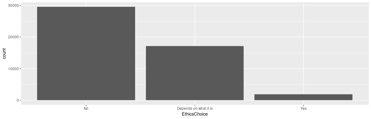
You might agree that with a question containing the phrase a purpose or product that you consider extremely unethical, the answer “depends on what it is” feels closer to “yes” than to “no.” If that seems like too skeptical a thought, it’s still the only binarization that achieves a sensible split.
data <- data %>% mutate(
  EthicsChoice = if_else(as.numeric(EthicsChoice) == 2, 1, 0)
  )
Looking at our second target variable, JobSatisfaction:
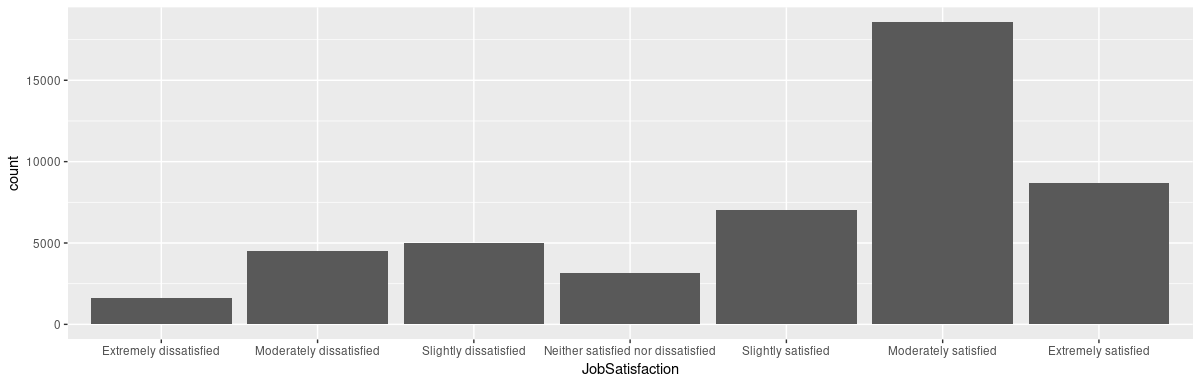
We think that given the mode at “moderately satisfied,” a sensible way to binarize is a split into “moderately satisfied” and “extremely satisfied” on one side, all remaining options on the other:
data <- data %>% mutate(
  JobSatisfaction = if_else(as.numeric(JobSatisfaction) > 5, 1, 0)
  )
Predictors
Among the predictors, FormalEducation, UndergradMajor and OperatingSystem look pretty harmless - we already turned them into factors so it should be straightforward to one-hot-encode them. For curiosity’s sake, let’s look at how they’re distributed:
  FormalEducation                                        count
  <fct>                                                  <int>
1 Bachelor’s degree (BA, BS, B.Eng., etc.)               25558
2 Master’s degree (MA, MS, M.Eng., MBA, etc.)            12865
3 Some college/university study without earning a degree  6474
4 Associate degree                                        1595
5 Other doctoral degree (Ph.D, Ed.D., etc.)               1395
6 Professional degree (JD, MD, etc.) 723 UndergradMajor count
<fct> <int>
1 Computer science, computer engineering, or software engineering 30931
2 Another engineering discipline (ex. civil, electrical, mechani… 4179
3 Information systems, information technology, or system adminis… 3953
4 A natural science (ex. biology, chemistry, physics) 2046
5 Mathematics or statistics 1853
6 Web development or web design 1171
7 A business discipline (ex. accounting, finance, marketing) 1166
8 A humanities discipline (ex. literature, history, philosophy) 1104
9 A social science (ex. anthropology, psychology, political scie… 888
10 Fine arts or performing arts (ex. graphic design, music, studi… 791
11 I never declared a major 398
12 A health science (ex. nursing, pharmacy, radiology) 130 OperatingSystem count
<fct> <int>
1 Windows 23470
2 MacOS 14216
3 Linux-based 10837
4 BSD/Unix 87LanguageWorkedWith, on the other hand, contains sequences of programming languages, concatenated by semicolon.
One way to unpack these is using Keras’ text_tokenizer.
language_tokenizer <- text_tokenizer(split = ";", filters = "")
language_tokenizer %>% fit_text_tokenizer(data$LanguageWorkedWith)
We have 38 languages overall. Actual usage counts aren’t too surprising:
                   name count
1            javascript 35224
2                  html 33287
3                   css 31744
4                   sql 29217
5                  java 21503
6            bash/shell 20997
7                python 18623
8                    c# 17604
9                   php 13843
10                  c++ 10846
11           typescript  9551
12                    c  9297
13                 ruby  5352
14                swift  4014
15                   go  3784
16          objective-c  3651
17               vb.net  3217
18                    r  3049
19             assembly  2699
20               groovy  2541
21                scala  2475
22               matlab  2465
23               kotlin  2305
24                  vba  2298
25                 perl  2164
26       visual basic 6  1729
27         coffeescript  1711
28                  lua  1556
29 delphi/object pascal  1174
30                 rust  1132
31              haskell  1058
32                   f#   764
33              clojure   696
34               erlang   560
35                cobol   317
36                ocaml   216
37                julia   215
38                 hack    94
Now language_tokenizer will nicely create a one-hot representation of the multiple-choice column.
langs <- language_tokenizer %>%
  texts_to_matrix(data$LanguageWorkedWith, mode = "count")
langs[1:3, ]
> langs[1:3, ]
[,1] [,2] [,3] [,4] [,5] [,6] [,7] [,8] [,9] [,10] [,11] [,12] [,13] [,14] [,15] [,16] [,17] [,18] [,19] [,20] [,21]
[1,] 0 1 1 1 0 0 0 1 0 0 0 0 0 0 0 0 0 0 0 0 0
[2,] 0 1 0 0 0 0 1 1 0 0 0 0 0 0 0 0 0 0 0 0 0
[3,] 0 0 0 0 1 1 1 0 0 0 1 0 1 0 0 0 0 0 1 0 0
[,22] [,23] [,24] [,25] [,26] [,27] [,28] [,29] [,30] [,31] [,32] [,33] [,34] [,35] [,36] [,37] [,38] [,39]
[1,] 0 0 0 0 0 0 0 0 0 0 0 0 0 0 0 0 0 0
[2,] 0 0 0 0 0 0 0 0 0 0 0 0 0 0 0 0 0 0
[3,] 0 1 0 0 0 0 0 0 0 0 0 0 0 0 0 0 0 0We can simply append these columns to the dataframe (and do a little cleanup):
We still have the AssessJob[n] columns to deal with. Here, StackOverflow had people rank what’s important to them about a job. These are the features that were to be ranked:
The industry that I’d be working in
The financial performance or funding status of the company or organization
The specific department or team I’d be working on
The languages, frameworks, and other technologies I’d be working with
The compensation and benefits offered
The office environment or company culture
The opportunity to work from home/remotely
Opportunities for professional development
The diversity of the company or organization
How widely used or impactful the product or service I’d be working on is
Columns AssessJob1 to AssessJob10 contain the respective ranks, that is, values between 1 and 10.
Based on introspection about the cognitive effort to actually establish an order among 10 items, we decided to pull out the three top-ranked features per person and treat them as equal. Technically, a first step extracts and concatenate these, yielding an intermediary result of e.g.
$ job_vals<fct> languages_frameworks;compensation;remote, industry;compensation;development, languages_frameworks;compensation;developmentdata <- data %>% mutate(
val_1 = if_else(
AssessJob1 == 1, "industry", if_else(
AssessJob2 == 1, "company_financial_status", if_else(
AssessJob3 == 1, "department", if_else(
AssessJob4 == 1, "languages_frameworks", if_else(
AssessJob5 == 1, "compensation", if_else(
AssessJob6 == 1, "company_culture", if_else(
AssessJob7 == 1, "remote", if_else(
AssessJob8 == 1, "development", if_else(
AssessJob10 == 1, "diversity", "impact"))))))))),
val_2 = if_else(
AssessJob1 == 2, "industry", if_else(
AssessJob2 == 2, "company_financial_status", if_else(
AssessJob3 == 2, "department", if_else(
AssessJob4 == 2, "languages_frameworks", if_else(
AssessJob5 == 2, "compensation", if_else(
AssessJob6 == 2, "company_culture", if_else(
AssessJob7 == 1, "remote", if_else(
AssessJob8 == 1, "development", if_else(
AssessJob10 == 1, "diversity", "impact"))))))))),
val_3 = if_else(
AssessJob1 == 3, "industry", if_else(
AssessJob2 == 3, "company_financial_status", if_else(
AssessJob3 == 3, "department", if_else(
AssessJob4 == 3, "languages_frameworks", if_else(
AssessJob5 == 3, "compensation", if_else(
AssessJob6 == 3, "company_culture", if_else(
AssessJob7 == 3, "remote", if_else(
AssessJob8 == 3, "development", if_else(
AssessJob10 == 3, "diversity", "impact")))))))))
)
data <- data %>% mutate(
job_vals = paste(val_1, val_2, val_3, sep = ";") %>% factor()
)
data <- data %>% select(
-c(starts_with("AssessJob"), starts_with("val_"))
)Now that column looks exactly like LanguageWorkedWith looked before, so we can use the same method as above to produce a one-hot-encoded version.
values_tokenizer <- text_tokenizer(split = ";", filters = "")
values_tokenizer %>% fit_text_tokenizer(data$job_vals)
So what actually do respondents value most?
                      name count
1              compensation 27020
2      languages_frameworks 24216
3           company_culture 20432
4               development 15981
5                    impact 14869
6                department 10452
7                    remote 10396
8                  industry  8294
9                 diversity  7594
10 company_financial_status  6576
Using the same method as above
we end up with a dataset that looks like this
> data %>% glimpse()
Observations: 48,610
Variables: 53
$ FormalEducation          <fct> Bachelor’s degree (BA, BS, B.Eng., etc.), Bach...
$ UndergradMajor           <fct> Mathematics or statistics, A natural science (...
$ OperatingSystem          <fct> Linux-based, Linux-based, Windows, Linux-based...
$ JS                       <dbl> 1, 0, 0, 1, 0, 0, 1, 1, 1, 0, 0, 0, 1, 1, 0, 0...
$ EC                       <dbl> 0, 1, 0, 1, 1, 1, 0, 1, 0, 0, 0, 0, 0, 1, 0, 0...
$ javascript               <dbl> 1, 1, 0, 1, 1, 1, 1, 0, 0, 0, 1, 1, 1, 1, 0, 1...
$ html                     <dbl> 1, 0, 0, 1, 1, 1, 1, 0, 1, 0, 1, 1, 1, 1, 1, 1...
$ css                      <dbl> 1, 0, 0, 1, 1, 1, 1, 0, 1, 0, 1, 1, 1, 1, 0, 1...
$ sql                      <dbl> 0, 0, 1, 0, 0, 0, 1, 0, 1, 1, 1, 1, 1, 1, 1, 1...
$ java                     <dbl> 0, 0, 1, 1, 0, 0, 0, 1, 0, 0, 0, 1, 1, 0, 0, 1...
$ `bash/shell`             <dbl> 0, 1, 1, 0, 0, 0, 1, 0, 1, 0, 0, 0, 0, 0, 1, 1...
$ python                   <dbl> 1, 1, 0, 1, 0, 0, 1, 0, 0, 1, 0, 0, 0, 0, 1, 0...
$ `c#`                     <dbl> 0, 0, 0, 0, 0, 0, 0, 0, 1, 0, 1, 0, 1, 1, 0, 0...
$ php                      <dbl> 0, 0, 0, 0, 0, 0, 0, 0, 0, 0, 1, 1, 1, 0, 0, 1...
$ `c++`                    <dbl> 0, 0, 1, 0, 0, 0, 0, 0, 0, 1, 0, 0, 0, 0, 0, 0...
$ typescript               <dbl> 0, 0, 0, 1, 0, 1, 0, 0, 0, 0, 0, 1, 0, 0, 0, 1...
$ c                        <dbl> 0, 0, 1, 0, 0, 0, 0, 0, 0, 1, 0, 0, 0, 0, 0, 0...
$ ruby                     <dbl> 0, 0, 0, 0, 0, 0, 1, 0, 0, 0, 0, 0, 0, 0, 0, 0...
$ swift                    <dbl> 0, 0, 0, 0, 0, 0, 0, 0, 0, 1, 0, 0, 0, 0, 0, 1...
$ go                       <dbl> 0, 0, 0, 0, 0, 0, 1, 0, 0, 1, 0, 0, 0, 0, 0, 0...
$ `objective-c`            <dbl> 0, 0, 0, 0, 0, 0, 0, 0, 0, 0, 0, 0, 0, 0, 0, 0...
$ vb.net                   <dbl> 0, 0, 0, 0, 0, 0, 0, 0, 0, 0, 0, 0, 0, 0, 0, 0...
$ r                        <dbl> 0, 0, 1, 0, 0, 0, 0, 0, 0, 0, 0, 0, 0, 0, 0, 0...
$ assembly                 <dbl> 0, 0, 0, 0, 0, 0, 1, 0, 0, 0, 0, 0, 0, 0, 0, 0...
$ groovy                   <dbl> 0, 0, 0, 0, 0, 0, 0, 0, 0, 0, 0, 0, 0, 0, 0, 0...
$ scala                    <dbl> 0, 0, 0, 0, 0, 0, 0, 0, 0, 0, 0, 0, 0, 0, 0, 0...
$ matlab                   <dbl> 0, 0, 1, 0, 0, 0, 0, 0, 0, 0, 0, 0, 0, 0, 0, 0...
$ kotlin                   <dbl> 0, 0, 0, 0, 0, 0, 0, 0, 0, 0, 0, 0, 0, 0, 0, 0...
$ vba                      <dbl> 0, 0, 0, 0, 0, 0, 0, 0, 0, 0, 0, 0, 0, 0, 0, 0...
$ perl                     <dbl> 0, 0, 0, 0, 0, 0, 0, 0, 0, 0, 0, 0, 0, 0, 0, 0...
$ `visual basic 6`         <dbl> 0, 0, 0, 0, 0, 0, 0, 0, 0, 0, 0, 0, 0, 0, 0, 0...
$ coffeescript             <dbl> 0, 0, 0, 0, 0, 0, 1, 0, 0, 0, 0, 0, 0, 0, 0, 0...
$ lua                      <dbl> 0, 0, 0, 0, 0, 0, 1, 0, 0, 0, 0, 0, 0, 0, 0, 0...
$ `delphi/object pascal`   <dbl> 0, 0, 0, 0, 0, 0, 0, 0, 0, 0, 0, 0, 0, 0, 0, 0...
$ rust                     <dbl> 0, 0, 0, 0, 0, 0, 0, 0, 0, 0, 0, 0, 0, 0, 0, 0...
$ haskell                  <dbl> 0, 0, 0, 0, 0, 0, 0, 0, 0, 0, 0, 0, 0, 0, 0, 0...
$ `f#`                     <dbl> 0, 0, 0, 0, 0, 0, 0, 0, 0, 0, 0, 0, 0, 0, 0, 0...
$ clojure                  <dbl> 0, 0, 0, 0, 0, 0, 0, 0, 0, 0, 0, 0, 0, 0, 0, 0...
$ erlang                   <dbl> 0, 0, 0, 0, 0, 0, 1, 0, 0, 0, 0, 0, 0, 0, 0, 0...
$ cobol                    <dbl> 0, 0, 0, 0, 0, 0, 0, 0, 0, 0, 0, 0, 0, 0, 0, 0...
$ ocaml                    <dbl> 0, 0, 0, 0, 0, 0, 0, 0, 0, 0, 0, 0, 0, 0, 0, 0...
$ julia                    <dbl> 0, 0, 0, 0, 0, 0, 0, 0, 0, 0, 0, 0, 0, 0, 0, 0...
$ hack                     <dbl> 0, 0, 0, 0, 0, 0, 0, 0, 0, 0, 0, 0, 0, 0, 0, 0...
$ compensation             <dbl> 1, 1, 1, 1, 1, 0, 1, 1, 1, 1, 0, 0, 1, 0, 1, 0...
$ languages_frameworks     <dbl> 1, 0, 1, 0, 0, 1, 0, 0, 1, 1, 0, 0, 0, 1, 0, 0...
$ company_culture          <dbl> 0, 0, 0, 1, 0, 0, 0, 0, 0, 0, 0, 0, 0, 0, 0, 0...
$ development              <dbl> 0, 1, 1, 0, 0, 1, 0, 0, 0, 0, 0, 1, 1, 1, 1, 0...
$ impact                   <dbl> 0, 0, 0, 1, 1, 0, 1, 0, 1, 0, 0, 1, 0, 1, 0, 1...
$ department               <dbl> 0, 0, 0, 0, 0, 0, 0, 1, 0, 0, 0, 0, 0, 0, 0, 0...
$ remote                   <dbl> 1, 0, 0, 0, 0, 0, 0, 0, 0, 1, 2, 0, 1, 0, 1, 0...
$ industry                 <dbl> 0, 1, 0, 0, 0, 0, 0, 0, 0, 0, 1, 1, 0, 0, 0, 1...
$ diversity                <dbl> 0, 0, 0, 0, 0, 1, 0, 1, 0, 0, 0, 0, 0, 0, 0, 0...
$ company_financial_status <dbl> 0, 0, 0, 0, 1, 0, 1, 0, 0, 0, 0, 0, 0, 0, 0, 1...
which we further reduce to a design matrix X removing the binarized target variables
From here on, different actions will ensue depending on whether we choose the road of working with a one-hot model or an embeddings model of the predictors.
There is one other thing though to be done before: We want to work with the same train-test split in both cases.
One-hot model
Given this is a post about embeddings, why show a one-hot model? First, for instructional reasons - you don’t see many of examples of deep learning on categorical data in the wild. Second, … but we’ll turn to that after having shown both models.
For the one-hot model, all that remains to be done is using Keras’ to_categorical on the three remaining variables that are not yet in one-hot form.
X_one_hot <- X %>% map_if(is.factor, ~ as.integer(.x) - 1) %>%
  map_at("FormalEducation", ~ to_categorical(.x) %>%
           array_reshape(c(length(.x), length(levels(data$FormalEducation))))) %>%
  map_at("UndergradMajor", ~ to_categorical(.x) %>%
           array_reshape(c(length(.x), length(levels(data$UndergradMajor))))) %>%
  map_at("OperatingSystem", ~ to_categorical(.x) %>%
           array_reshape(c(length(.x), length(levels(data$OperatingSystem))))) %>%
  abind::abind(along = 2)
We divide up our dataset into train and validation parts
and define a pretty straightforward MLP.
model <- keras_model_sequential() %>%
layer_dense(
units = 128,
activation = "selu"
) %>%
layer_dropout(0.5) %>%
layer_dense(
units = 128,
activation = "selu"
) %>%
layer_dropout(0.5) %>%
layer_dense(
units = 128,
activation = "selu"
) %>%
layer_dropout(0.5) %>%
layer_dense(
units = 128,
activation = "selu"
) %>%
layer_dropout(0.5) %>%
layer_dense(units = 1, activation = "sigmoid")
model %>% compile(
loss = "binary_crossentropy",
optimizer = "adam",
metrics = "accuracy"
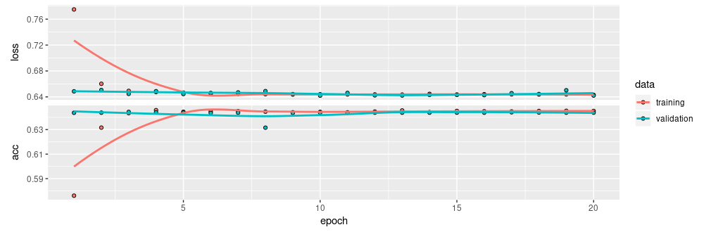
)Training this model:
…results in an accuracy on the validation set of 0.64 - not an impressive number per se, but interesting given the small amount of predictors and the choice of target variable.3
Embeddings model
In the embeddings model, we don’t need to use to_categorical on the remaining factors, as embedding layers can work with integer input data. We thus just convert the factors to integers:
Now for the model. Effectively we have five groups of entities here: formal education, undergrad major, operating system, languages worked with, and highest-counting values with respect to jobs. Each of these groups get embedded separately, so we need to use the Keras functional API and declare five different inputs.
input_fe <- layer_input(shape = 1)        # formal education, encoded as integer
input_um <- layer_input(shape = 1)        # undergrad major, encoded as integer
input_os <- layer_input(shape = 1)        # operating system, encoded as integer
input_langs <- layer_input(shape = 38)    # languages worked with, multi-hot-encoded
input_vals <- layer_input(shape = 10)     # values, multi-hot-encoded
Having embedded them separately, we concatenate the outputs for further common processing.
concat <- layer_concatenate(
  list(
    input_fe %>%
      layer_embedding(
        input_dim = length(levels(data$FormalEducation)),
        output_dim = 64,
        name = "fe"
      ) %>%
      layer_flatten(),
    input_um %>%
      layer_embedding(
        input_dim = length(levels(data$UndergradMajor)),
        output_dim = 64,
        name = "um"
      ) %>%
      layer_flatten(),
    input_os %>%
      layer_embedding(
        input_dim = length(levels(data$OperatingSystem)),
        output_dim = 64,
        name = "os"
      ) %>%
      layer_flatten(),
    input_langs %>%
       layer_embedding(input_dim = 38, output_dim = 256,
                       name = "langs")%>%
       layer_flatten(),
    input_vals %>%
      layer_embedding(input_dim = 10, output_dim = 128,
                      name = "vals")%>%
      layer_flatten()
  )
)

output <- concat %>%
  layer_dense(
    units = 128,
    activation = "relu"
  ) %>%
  layer_dropout(0.5) %>%
  layer_dense(
    units = 128,
    activation = "relu"
  ) %>%
  layer_dropout(0.5) %>%
  layer_dense(
    units = 128,
    activation = "relu"
  ) %>%
  layer_dense(
    units = 128,
    activation = "relu"
  ) %>%
  layer_dropout(0.5) %>%
  layer_dense(units = 1, activation = "sigmoid")
So there go model definition and compilation:
Now to pass the data to the model, we need to chop it up into ranges of columns matching the inputs.
y_train <- data$EthicsChoice[train_indices] %>% as.matrix()
y_valid <- data$EthicsChoice[-train_indices] %>% as.matrix()

x_train <-
  list(
    X_embed[train_indices, 1, drop = FALSE] %>% as.matrix() ,
    X_embed[train_indices , 2, drop = FALSE] %>% as.matrix(),
    X_embed[train_indices , 3, drop = FALSE] %>% as.matrix(),
    X_embed[train_indices , 4:41, drop = FALSE] %>% as.matrix(),
    X_embed[train_indices , 42:51, drop = FALSE] %>% as.matrix()
  )
x_valid <- list(
  X_embed[-train_indices, 1, drop = FALSE] %>% as.matrix() ,
  X_embed[-train_indices , 2, drop = FALSE] %>% as.matrix(),
  X_embed[-train_indices , 3, drop = FALSE] %>% as.matrix(),
  X_embed[-train_indices , 4:41, drop = FALSE] %>% as.matrix(),
  X_embed[-train_indices , 42:51, drop = FALSE] %>% as.matrix()
)
And we’re ready to train.
Using the same train-test split as before, this results in an accuracy of … ~0.64 (just as before). Now we said from the start that using embeddings could serve different purposes, and that in this first use case, we wanted to demonstrate their use for extracting latent relationships. And in any case you could argue that the task is too hard - probably there just is not much of a relationship between the predictors we chose and the target.
But this also warrants a more general comment. With all current enthusiasm about using embeddings on tabular data, we are not aware of any systematic comparisons with one-hot-encoded data as regards the actual effect on performance, nor do we know of systematic analyses under what circumstances embeddings will probably be of help. Our working hypothesis is that in the setup we chose, the dimensionality of the original data is so low that the information can simply be encoded “as is” by the network - as long as we create it with sufficient capacity. Our second use case will therefore use data where - hopefully - this won’t be the case.
But before, let’s get to the main purpose of this use case: How can we extract those latent relationships from the network?
Extracting relationships from the learned embeddings
We’ll show the code here for the job values embeddings, - it is directly transferable to the other ones.
The embeddings, that’s just the weight matrix of the respective layer, of dimension number of different values times embedding size.
We can then perform dimensionality reduction on the raw values, e.g., PCA
and plot the results.
This is what we get (displaying four of the five variables we used embeddings on):
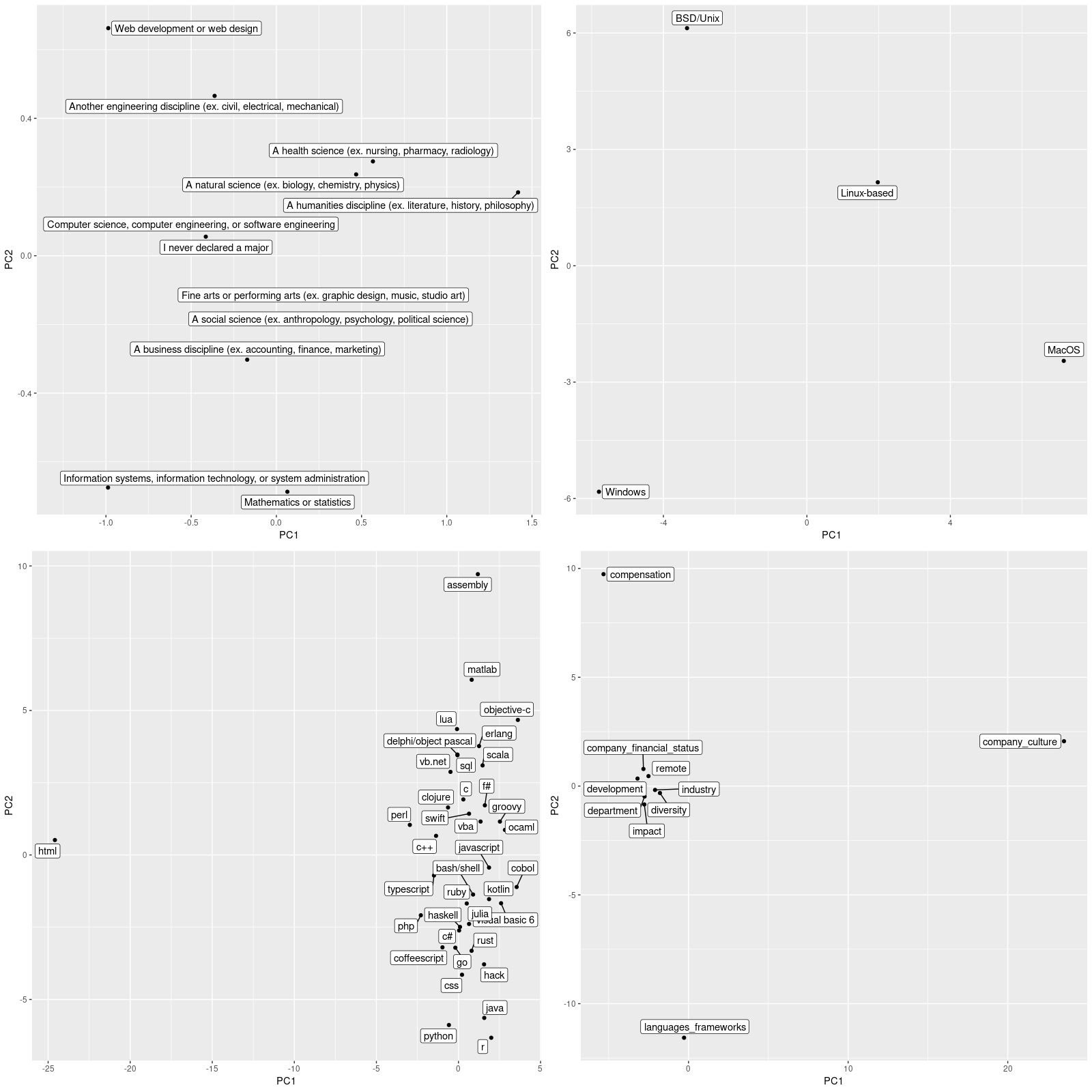
Now we’ll definitely refrain from taking this too seriously, given the modest accuracy on the prediction task that lead to these embedding matrices.4 Certainly when assessing the obtained factorization, performance on the main task has to be taken into account.
But we’d like to point out something else too: In contrast to unsupervised and semi-supervised techniques like PCA or autoencoders, we made use of an extraneous variable (the ethical behavior to be predicted). So any learned relationships are never “absolute,” but always to be seen in relation to the way they were learned. This is why we chose an additional target variable, JobSatisfaction, so we could compare the embeddings learned on two different tasks. We won’t refer the concrete results here as accuracy turned out to be even lower than with EthicsChoice. We do, however, want to stress this inherent difference to representations learned by, e.g., autoencoders.
Now let’s address the second use case.
Embedding for profit (improving accuracy)
Our second task here is about fraud detection. The dataset is contained in the DMwR2 package and is called sales:
data(sales, package = "DMwR2")
sales
# A tibble: 401,146 x 5
ID Prod Quant Val Insp
<fct> <fct> <int> <dbl> <fct>
1 v1 p1 182 1665 unkn
2 v2 p1 3072 8780 unkn
3 v3 p1 20393 76990 unkn
4 v4 p1 112 1100 unkn
5 v3 p1 6164 20260 unkn
6 v5 p2 104 1155 unkn
7 v6 p2 350 5680 unkn
8 v7 p2 200 4010 unkn
9 v8 p2 233 2855 unkn
10 v9 p2 118 1175 unkn
# ... with 401,136 more rowsEach row indicates a transaction reported by a salesperson, - ID being the salesperson ID, Prod a product ID, Quant the quantity sold, Val the amount of money it was sold for, and Insp indicating one of three possibilities: (1) the transaction was examined and found fraudulent, (2) it was examined and found okay, and (3) it has not been examined (the vast majority of cases).
While this dataset “cries” for semi-supervised techniques (to make use of the overwhelming amount of unlabeled data), we want to see if using embeddings can help us improve accuracy on a supervised task.
We thus recklessly throw away incomplete data as well as all unlabeled entries
which leaves us with 15546 transactions.
One-hot model
Now we prepare the data for the one-hot model we want to compare against:
- With 2821 levels, salesperson
IDis far too high-dimensional to work well with one-hot encoding, so we completely drop that column. - Product id (
Prod) has “just” 797 levels, but with one-hot-encoding, that still results in significant memory demand. We thus zoom in on the 500 top-sellers. - The continuous variables
QuantandValare normalized to values between 0 and 1 so they fit with the one-hot-encodedProd.
sales_1hot <- sales

normalize <- function(x) {
  (x - min(x)) / (max(x) - min(x))
}

top_n <- 500
top_prods <- sales_1hot %>%
  group_by(Prod) %>%
  summarise(cnt = n()) %>%
  arrange(desc(cnt)) %>%
  head(top_n) %>%
  select(Prod) %>%
  pull()
sales_1hot <- droplevels(sales_1hot %>% filter(Prod %in% top_prods))

sales_1hot <- sales_1hot %>%
  select(-ID) %>%
  map_if(is.factor, ~ as.integer(.x) - 1) %>%
  map_at("Prod", ~ to_categorical(.x) %>% array_reshape(c(length(.x), top_n))) %>%
  map_at("Quant", ~ normalize(.x) %>% array_reshape(c(length(.x), 1))) %>%
  map_at("Val", ~ normalize(.x) %>% array_reshape(c(length(.x), 1))) %>%
  abind(along = 2)
We then perform the usual train-test split.
For classification on this dataset, which will be the baseline to beat?
[[1]]
        0
0.9393547

[[2]]
        0
0.9384437
So if we don’t get beyond 94% accuracy on both training and validation sets, we may just as well predict “okay” for every transaction.
Here then is the model, plus the training routine and evaluation:
model <- keras_model_sequential() %>%
  layer_dense(units = 256, activation = "selu") %>%
  layer_dropout(dropout_rate) %>%
  layer_dense(units = 256, activation = "selu") %>%
  layer_dropout(dropout_rate) %>%
  layer_dense(units = 256, activation = "selu") %>%
  layer_dropout(dropout_rate) %>%
  layer_dense(units = 256, activation = "selu") %>%
  layer_dropout(dropout_rate) %>%
  layer_dense(units = 1, activation = "sigmoid")

model %>% compile(loss = "binary_crossentropy", optimizer = "adam", metrics = c("accuracy"))

model %>% fit(
  X_train,
  y_train,
  validation_data = list(X_valid, y_valid),
  class_weights = list("0" = 0.1, "1" = 0.9),
  batch_size = 128,
  epochs = 200
)

model %>% evaluate(X_train, y_train, batch_size = 100)
model %>% evaluate(X_valid, y_valid, batch_size = 100)
This model achieved optimal validation accuracy at a dropout rate of 0.2. At that rate, training accuracy was 0.9761, and validation accuracy was 0.9507. At all dropout rates lower than 0.7, validation accuracy did indeed surpass the majority vote baseline.
Can we further improve performance by embedding the product id?
Embeddings model
For better comparability, we again discard salesperson information and cap the number of different products at 500. Otherwise, data preparation goes as expected for this model:
sales_embed <- sales

top_prods <- sales_embed %>%
  group_by(Prod) %>%
  summarise(cnt = n()) %>%
  arrange(desc(cnt)) %>%
  head(top_n) %>%
  select(Prod) %>%
  pull()

sales_embed <- droplevels(sales_embed %>% filter(Prod %in% top_prods))

sales_embed <- sales_embed %>%
  select(-ID) %>%
  mutate_if(is.factor, ~ as.integer(.x) - 1) %>%
  mutate(Quant = scale(Quant)) %>%
  mutate(Val = scale(Val))

X_train <- sales_embed[train_indices, 1:3] %>% as.matrix()
y_train <-  sales_embed[train_indices, 4] %>% as.matrix()

X_valid <- sales_embed[-train_indices, 1:3] %>% as.matrix()
y_valid <-  sales_embed[-train_indices, 4] %>% as.matrix()
The model we define is as similar as possible to the one-hot alternative:
prod_input <- layer_input(shape = 1)
cont_input <- layer_input(shape = 2)

prod_embed <- prod_input %>%
  layer_embedding(input_dim = sales_embed$Prod %>% max() + 1,
                  output_dim = 256
                  ) %>%
  layer_flatten()
cont_dense <- cont_input %>% layer_dense(units = 256, activation = "selu")

output <- layer_concatenate(
  list(prod_embed, cont_dense)) %>%
  layer_dropout(dropout_rate) %>%
  layer_dense(units = 256, activation = "selu") %>%
  layer_dropout(dropout_rate) %>%
  layer_dense(units = 256, activation = "selu") %>%
  layer_dropout(dropout_rate) %>%
  layer_dense(units = 256, activation = "selu") %>%
  layer_dropout(dropout_rate) %>%
  layer_dense(units = 1, activation = "sigmoid")

model <- keras_model(inputs = list(prod_input, cont_input), outputs = output)

model %>% compile(loss = "binary_crossentropy", optimizer = "adam", metrics = "accuracy")

model %>% fit(
  list(X_train[ , 1], X_train[ , 2:3]),
  y_train,
  validation_data = list(list(X_valid[ , 1], X_valid[ , 2:3]), y_valid),
  class_weights = list("0" = 0.1, "1" = 0.9),
  batch_size = 128,
  epochs = 200
)

model %>% evaluate(list(X_train[ , 1], X_train[ , 2:3]), y_train)
model %>% evaluate(list(X_valid[ , 1], X_valid[ , 2:3]), y_valid)
This time, accuracies are in fact higher: At the optimal dropout rate (0.3 in this case), training resp. validation accuracy are at 0.9913 and 0.9666, respectively. Quite a difference!
So why did we choose this dataset? In contrast to our previous dataset, here the categorical variable is high-dimensional, so well suited for compression and densification. It is interesting that we can make such good use of an ID without knowing what it stands for!
Conclusion
In this post, we’ve shown two use cases of embeddings in “simple” tabular data. As stated in the introduction, to us, embeddings are what you make of them. In that vein, if you’ve used embeddings to accomplish things that mattered to your task at hand, please comment and tell us about it!
We did think it prudent though to omit variables like country, ethnicity or gender.↩︎
at least given the way we binarized answers (more on that soon)↩︎
As usual when not working with one the “flagship areas” of deep learning, comparisons against other machine learning methods would be interesting. We did, however, not want to further elongate the post, nor distract from its main focus, namely, the use of embeddings with categorical data.↩︎
No, no, of course we’re not implying that for programming languages, the second principal component, with R and assembly at its extremes, stands for high-level vs. low-level language here.↩︎