The recent announcement of TensorFlow 2.0 names eager execution as the number one central feature of the new major version. What does this mean for R users? As demonstrated in our recent post on neural machine translation, you can use eager execution from R now already, in combination with Keras custom models and the datasets API. It’s good to know you can use it - but why should you? And in which cases?
In this and a few upcoming posts, we want to show how eager execution can make developing models a lot easier. The degree of simplication will depend on the task - and just how much easier you’ll find the new way might also depend on your experience using the functional API to model more complex relationships. Even if you think that GANs, encoder-decoder architectures, or neural style transfer didn’t pose any problems before the advent of eager execution, you might find that the alternative is a better fit to how we humans mentally picture problems.
For this post, we are porting code from a recent Google Colaboratory notebook implementing the DCGAN architecture.(Radford, Metz, and Chintala 2015) No prior knowledge of GANs is required - we’ll keep this post practical (no maths) and focus on how to achieve your goal, mapping a simple and vivid concept into an astonishingly small number of lines of code.
As in the post on machine translation with attention, we first have to cover some prerequisites. By the way, no need to copy out the code snippets - you’ll find the complete code in eager_dcgan.R).
Prerequisites
The code in this post depends on the newest CRAN versions of several of the TensorFlow R packages. You can install these packages as follows:
install.packages(c("tensorflow", "keras", "tfdatasets"))You should also be sure that you are running the very latest version of TensorFlow (v1.10), which you can install like so:
library(tensorflow)
install_tensorflow()
There are additional requirements for using TensorFlow eager execution. First, we need to call tfe_enable_eager_execution() right at the beginning of the program. Second, we need to use the implementation of Keras included in TensorFlow, rather than the base Keras implementation.
We’ll also use the tfdatasets package for our input pipeline. So we end up with the following preamble to set things up:
library(keras)
use_implementation("tensorflow")

library(tensorflow)
tfe_enable_eager_execution(device_policy = "silent")

library(tfdatasets)
That’s it. Let’s get started.
So what’s a GAN?
GAN stands for Generative Adversarial Network(Goodfellow et al. 2014). It is a setup of two agents, the generator and the discriminator, that act against each other (thus, adversarial). It is generative because the goal is to generate output (as opposed to, say, classification or regression).
In human learning, feedback - direct or indirect - plays a central role. Say we wanted to forge a banknote (as long as those still exist). Assuming we can get away with unsuccessful trials, we would get better and better at forgery over time. Optimizing our technique, we would end up rich. This concept of optimizing from feedback is embodied in the first of the two agents, the generator. It gets its feedback from the discriminator, in an upside-down way: If it can fool the discriminator, making it believe that the banknote was real, all is fine; if the discriminator notices the fake, it has to do things differently. For a neural network, that means it has to update its weights.
How does the discriminator know what is real and what is fake? It too has to be trained, on real banknotes (or whatever the kind of objects involved) and the fake ones produced by the generator. So the complete setup is two agents competing, one striving to generate realistic-looking fake objects, and the other, to disavow the deception. The purpose of training is to have both evolve and get better, in turn causing the other to get better, too.
In this system, there is no objective minimum to the loss function: We want both components to learn and getter better “in lockstep,” instead of one winning out over the other. This makes optimization difficult. In practice therefore, tuning a GAN can seem more like alchemy than like science, and it often makes sense to lean on practices and “tricks” reported by others.
In this example, just like in the Google notebook we’re porting, the goal is to generate MNIST digits. While that may not sound like the most exciting task one could imagine, it lets us focus on the mechanics, and allows us to keep computation and memory requirements (comparatively) low.
Let’s load the data (training set needed only) and then, look at the first actor in our drama, the generator.
Training data
mnist <- dataset_mnist()
c(train_images, train_labels) %<-% mnist$train

train_images <- train_images %>%
  k_expand_dims() %>%
  k_cast(dtype = "float32")

# normalize images to [-1, 1] because the generator uses tanh activation
train_images <- (train_images - 127.5) / 127.5
Our complete training set will be streamed once per epoch:
buffer_size <- 60000
batch_size <- 256
batches_per_epoch <- (buffer_size / batch_size) %>% round()

train_dataset <- tensor_slices_dataset(train_images) %>%
  dataset_shuffle(buffer_size) %>%
  dataset_batch(batch_size)
This input will be fed to the discriminator only.
Generator
Both generator and discriminator are Keras custom models.
In contrast to custom layers, custom models allow you to construct models as independent units, complete with custom forward pass logic, backprop and optimization. The model-generating function defines the layers the model (self) wants assigned, and returns the function that implements the forward pass.
As we will soon see, the generator gets passed vectors of random noise for input. This vector is transformed to 3d (height, width, channels) and then, successively upsampled to the required output size of (28,28,3).
generator <-
  function(name = NULL) {
    keras_model_custom(name = name, function(self) {

      self$fc1 <- layer_dense(units = 7 * 7 * 64, use_bias = FALSE)
      self$batchnorm1 <- layer_batch_normalization()
      self$leaky_relu1 <- layer_activation_leaky_relu()
      self$conv1 <-
        layer_conv_2d_transpose(
          filters = 64,
          kernel_size = c(5, 5),
          strides = c(1, 1),
          padding = "same",
          use_bias = FALSE
        )
      self$batchnorm2 <- layer_batch_normalization()
      self$leaky_relu2 <- layer_activation_leaky_relu()
      self$conv2 <-
        layer_conv_2d_transpose(
          filters = 32,
          kernel_size = c(5, 5),
          strides = c(2, 2),
          padding = "same",
          use_bias = FALSE
        )
      self$batchnorm3 <- layer_batch_normalization()
      self$leaky_relu3 <- layer_activation_leaky_relu()
      self$conv3 <-
        layer_conv_2d_transpose(
          filters = 1,
          kernel_size = c(5, 5),
          strides = c(2, 2),
          padding = "same",
          use_bias = FALSE,
          activation = "tanh"
        )

      function(inputs, mask = NULL, training = TRUE) {
        self$fc1(inputs) %>%
          self$batchnorm1(training = training) %>%
          self$leaky_relu1() %>%
          k_reshape(shape = c(-1, 7, 7, 64)) %>%
          self$conv1() %>%
          self$batchnorm2(training = training) %>%
          self$leaky_relu2() %>%
          self$conv2() %>%
          self$batchnorm3(training = training) %>%
          self$leaky_relu3() %>%
          self$conv3()
      }
    })
  }
Discriminator
The discriminator is just a pretty normal convolutional network outputting a score. Here, usage of “score” instead of “probability” is on purpose: If you look at the last layer, it is fully connected, of size 1 but lacking the usual sigmoid activation. This is because unlike Keras’ loss_binary_crossentropy, the loss function we’ll be using here - tf$losses$sigmoid_cross_entropy - works with the raw logits, not the outputs of the sigmoid.
discriminator <-
  function(name = NULL) {
    keras_model_custom(name = name, function(self) {

      self$conv1 <- layer_conv_2d(
        filters = 64,
        kernel_size = c(5, 5),
        strides = c(2, 2),
        padding = "same"
      )
      self$leaky_relu1 <- layer_activation_leaky_relu()
      self$dropout <- layer_dropout(rate = 0.3)
      self$conv2 <-
        layer_conv_2d(
          filters = 128,
          kernel_size = c(5, 5),
          strides = c(2, 2),
          padding = "same"
        )
      self$leaky_relu2 <- layer_activation_leaky_relu()
      self$flatten <- layer_flatten()
      self$fc1 <- layer_dense(units = 1)

      function(inputs, mask = NULL, training = TRUE) {
        inputs %>% self$conv1() %>%
          self$leaky_relu1() %>%
          self$dropout(training = training) %>%
          self$conv2() %>%
          self$leaky_relu2() %>%
          self$flatten() %>%
          self$fc1()
      }
    })
  }
Setting the scene
Before we can start training, we need to create the usual components of a deep learning setup: the model (or models, in this case), the loss function(s), and the optimizer(s).
Model creation is just a function call, with a little extra on top:
generator <- generator()
discriminator <- discriminator()

# https://www.tensorflow.org/api_docs/python/tf/contrib/eager/defun
generator$call = tf$contrib$eager$defun(generator$call)
discriminator$call = tf$contrib$eager$defun(discriminator$call)
defun compiles an R function (once per different combination of argument shapes and non-tensor objects values)) into a TensorFlow graph, and is used to speed up computations. This comes with side effects and possibly unexpected behavior - please consult the documentation for the details. Here, we were mainly curious in how much of a speedup we might notice when using this from R - in our example, it resulted in a speedup of 130%.
On to the losses. Discriminator loss consists of two parts: Does it correctly identify real images as real, and does it correctly spot fake images as fake.
Here real_output and generated_output contain the logits returned from the discriminator - that is, its judgment of whether the respective images are fake or real.
discriminator_loss <- function(real_output, generated_output) {
  real_loss <- tf$losses$sigmoid_cross_entropy(
    multi_class_labels = k_ones_like(real_output),
    logits = real_output)
  generated_loss <- tf$losses$sigmoid_cross_entropy(
    multi_class_labels = k_zeros_like(generated_output),
    logits = generated_output)
  real_loss + generated_loss
}
Generator loss depends on how the discriminator judged its creations: It would hope for them all to be seen as real.
generator_loss <- function(generated_output) {
  tf$losses$sigmoid_cross_entropy(
    tf$ones_like(generated_output),
    generated_output)
}
Now we still need to define optimizers, one for each model.
discriminator_optimizer <- tf$train$AdamOptimizer(1e-4)
generator_optimizer <- tf$train$AdamOptimizer(1e-4)
Training loop
There are two models, two loss functions and two optimizers, but there is just one training loop, as both models depend on each other. The training loop will be over MNIST images streamed in batches, but we still need input to the generator - a random vector of size 100, in this case.
noise_dim <- 100Let’s take the training loop step by step. There will be an outer and an inner loop, one over epochs and one over batches. At the start of each epoch, we create a fresh iterator over the dataset:
for (epoch in seq_len(num_epochs)) {
  start <- Sys.time()
  total_loss_gen <- 0
  total_loss_disc <- 0
  iter <- make_iterator_one_shot(train_dataset)
Now for every batch we obtain from the iterator, we are calling the generator and having it generate images from random noise. Then, we’re calling the dicriminator on real images as well as the fake images just generated. For the discriminator, its relative outputs are directly fed into the loss function. For the generator, its loss will depend on how the discriminator judged its creations:
until_out_of_range({
  batch <- iterator_get_next(iter)
  noise <- k_random_normal(c(batch_size, noise_dim))
  with(tf$GradientTape() %as% gen_tape, { with(tf$GradientTape() %as% disc_tape, {
    generated_images <- generator(noise)
    disc_real_output <- discriminator(batch, training = TRUE)
    disc_generated_output <-
       discriminator(generated_images, training = TRUE)
    gen_loss <- generator_loss(disc_generated_output)
    disc_loss <- discriminator_loss(disc_real_output, disc_generated_output)
  }) })
Note that all model calls happen inside tf$GradientTape contexts. This is so the forward passes can be recorded and “played back” to back propagate the losses through the network.
Obtain the gradients of the losses to the respective models’ variables (tape$gradient) and have the optimizers apply them to the models’ weights (optimizer$apply_gradients):
gradients_of_generator <-
  gen_tape$gradient(gen_loss, generator$variables)
gradients_of_discriminator <-
  disc_tape$gradient(disc_loss, discriminator$variables)

generator_optimizer$apply_gradients(purrr::transpose(
  list(gradients_of_generator, generator$variables)
))
discriminator_optimizer$apply_gradients(purrr::transpose(
  list(gradients_of_discriminator, discriminator$variables)
))

total_loss_gen <- total_loss_gen + gen_loss
total_loss_disc <- total_loss_disc + disc_loss
This ends the loop over batches. Finish off the loop over epochs displaying current losses and saving a few of the generator’s artwork:
cat("Time for epoch ", epoch, ": ", Sys.time() - start, "\n")
cat("Generator loss: ", total_loss_gen$numpy() / batches_per_epoch, "\n")
cat("Discriminator loss: ", total_loss_disc$numpy() / batches_per_epoch, "\n\n")
if (epoch %% 10 == 0)
  generate_and_save_images(generator,
                           epoch,
                           random_vector_for_generation)
Here’s the training loop again, shown as a whole - even including the lines for reporting on progress, it is remarkably concise, and allows for a quick grasp of what is going on:
train <- function(dataset, epochs, noise_dim) {
  for (epoch in seq_len(num_epochs)) {
    start <- Sys.time()
    total_loss_gen <- 0
    total_loss_disc <- 0
    iter <- make_iterator_one_shot(train_dataset)

    until_out_of_range({
      batch <- iterator_get_next(iter)
      noise <- k_random_normal(c(batch_size, noise_dim))
      with(tf$GradientTape() %as% gen_tape, { with(tf$GradientTape() %as% disc_tape, {
        generated_images <- generator(noise)
        disc_real_output <- discriminator(batch, training = TRUE)
        disc_generated_output <-
          discriminator(generated_images, training = TRUE)
        gen_loss <- generator_loss(disc_generated_output)
        disc_loss <-
          discriminator_loss(disc_real_output, disc_generated_output)
      }) })

      gradients_of_generator <-
        gen_tape$gradient(gen_loss, generator$variables)
      gradients_of_discriminator <-
        disc_tape$gradient(disc_loss, discriminator$variables)

      generator_optimizer$apply_gradients(purrr::transpose(
        list(gradients_of_generator, generator$variables)
      ))
      discriminator_optimizer$apply_gradients(purrr::transpose(
        list(gradients_of_discriminator, discriminator$variables)
      ))

      total_loss_gen <- total_loss_gen + gen_loss
      total_loss_disc <- total_loss_disc + disc_loss

    })

    cat("Time for epoch ", epoch, ": ", Sys.time() - start, "\n")
    cat("Generator loss: ", total_loss_gen$numpy() / batches_per_epoch, "\n")
    cat("Discriminator loss: ", total_loss_disc$numpy() / batches_per_epoch, "\n\n")
    if (epoch %% 10 == 0)
      generate_and_save_images(generator,
                               epoch,
                               random_vector_for_generation)

  }
}
Here’s the function for saving generated images…
generate_and_save_images <- function(model, epoch, test_input) {
  predictions <- model(test_input, training = FALSE)
  png(paste0("images_epoch_", epoch, ".png"))
  par(mfcol = c(5, 5))
  par(mar = c(0.5, 0.5, 0.5, 0.5),
      xaxs = 'i',
      yaxs = 'i')
  for (i in 1:25) {
    img <- predictions[i, , , 1]
    img <- t(apply(img, 2, rev))
    image(
      1:28,
      1:28,
      img * 127.5 + 127.5,
      col = gray((0:255) / 255),
      xaxt = 'n',
      yaxt = 'n'
    )
  }
  dev.off()
}
… and we’re ready to go!
num_epochs <- 150
train(train_dataset, num_epochs, noise_dim)
Results
Here are some generated images after training for 150 epochs:
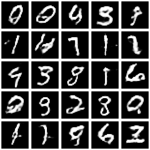
As they say, your results will most certainly vary!
Conclusion
While certainly tuning GANs will remain a challenge, we hope we were able to show that mapping concepts to code is not difficult when using eager execution. In case you’ve played around with GANs before, you may have found you needed to pay careful attention to set up the losses the right way, freeze the discriminator’s weights when needed, etc. This need goes away with eager execution. In upcoming posts, we will show further examples where using it makes model development easier.