How would your summer holiday’s photos look had Edvard Munch painted them? (Perhaps it’s better not to know). Let’s take a more comforting example: How would a nice, summarly river landscape look if painted by Katsushika Hokusai?
Style transfer on images is not new, but got a boost when Gatys, Ecker, and Bethge(Gatys, Ecker, and Bethge 2015) showed how to successfully do it with deep learning. The main idea is straightforward: Create a hybrid that is a tradeoff between the content image we want to manipulate, and a style image we want to imitate, by optimizing for maximal resemblance to both at the same time.
If you’ve read the chapter on neural style transfer from Deep Learning with R, you may recognize some of the code snippets that follow. However, there is an important difference: This post uses TensorFlow Eager Execution, allowing for an imperative way of coding that makes it easy to map concepts to code. Just like previous posts on eager execution on this blog, this is a port of a Google Colaboratory notebook that performs the same task in Python.
As usual, please make sure you have the required package versions installed. And no need to copy the snippets - you’ll find the complete code among the Keras examples.
Prerequisites
The code in this post depends on the most recent versions of several of the TensorFlow R packages. You can install these packages as follows:
install.packages(c("tensorflow", "keras", "tfdatasets"))You should also be sure that you are running the very latest version of TensorFlow (v1.10), which you can install like so:
library(tensorflow)
install_tensorflow()
There are additional requirements for using TensorFlow eager execution. First, we need to call tfe_enable_eager_execution() right at the beginning of the program. Second, we need to use the implementation of Keras included in TensorFlow, rather than the base Keras implementation.
Prerequisites behind us, let’s get started!
Input images
Here is our content image - replace by an image of your own:
# If you have enough memory on your GPU, no need to load the images
# at such small size.
# This is the size I found working for a 4G GPU.
img_shape <- c(128, 128, 3)

content_path <- "isar.jpg"

content_image <-  image_load(content_path, target_size = img_shape[1:2])
content_image %>%
  image_to_array() %>%
  `/`(., 255) %>%
  as.raster() %>%
  plot()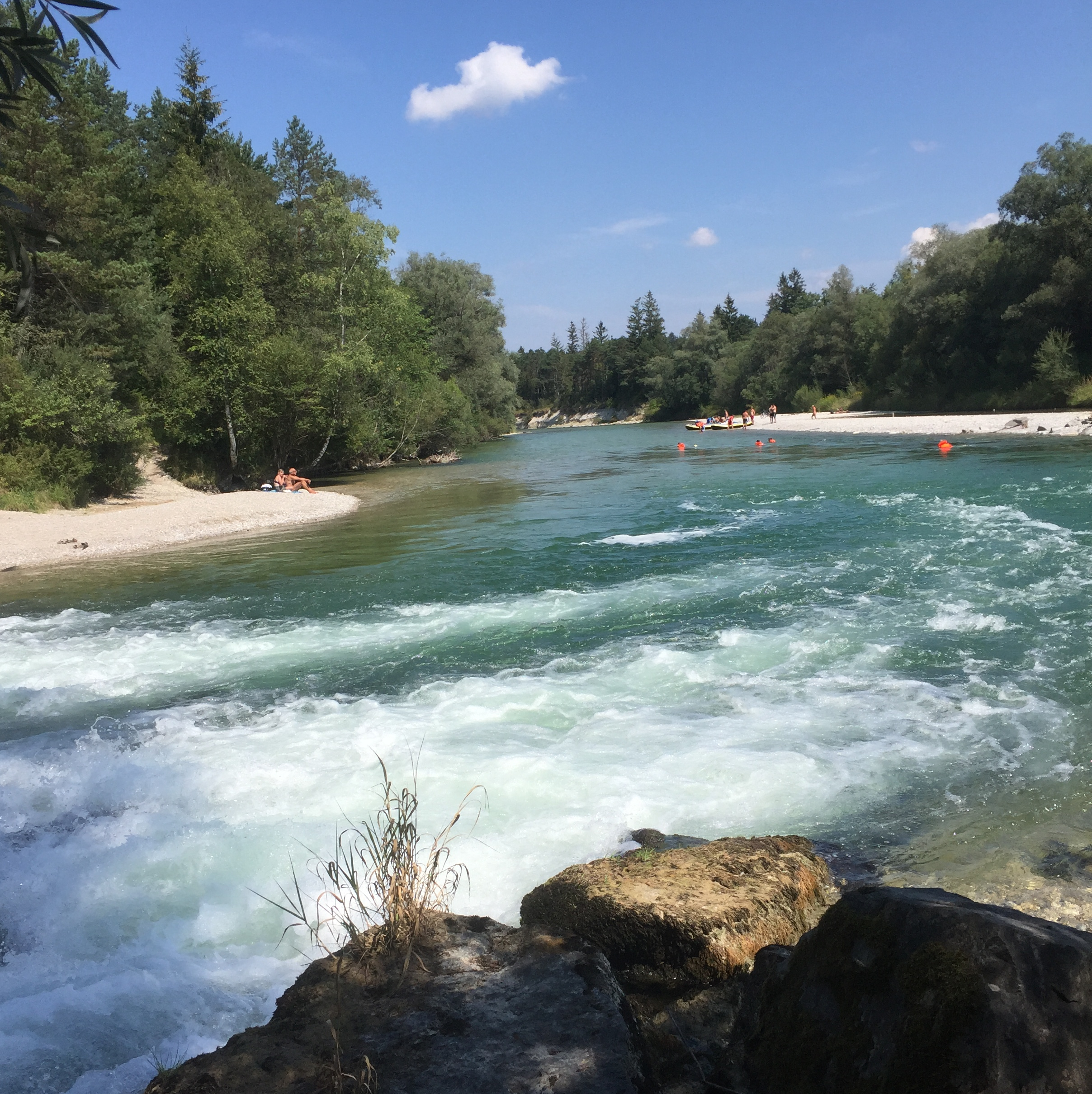
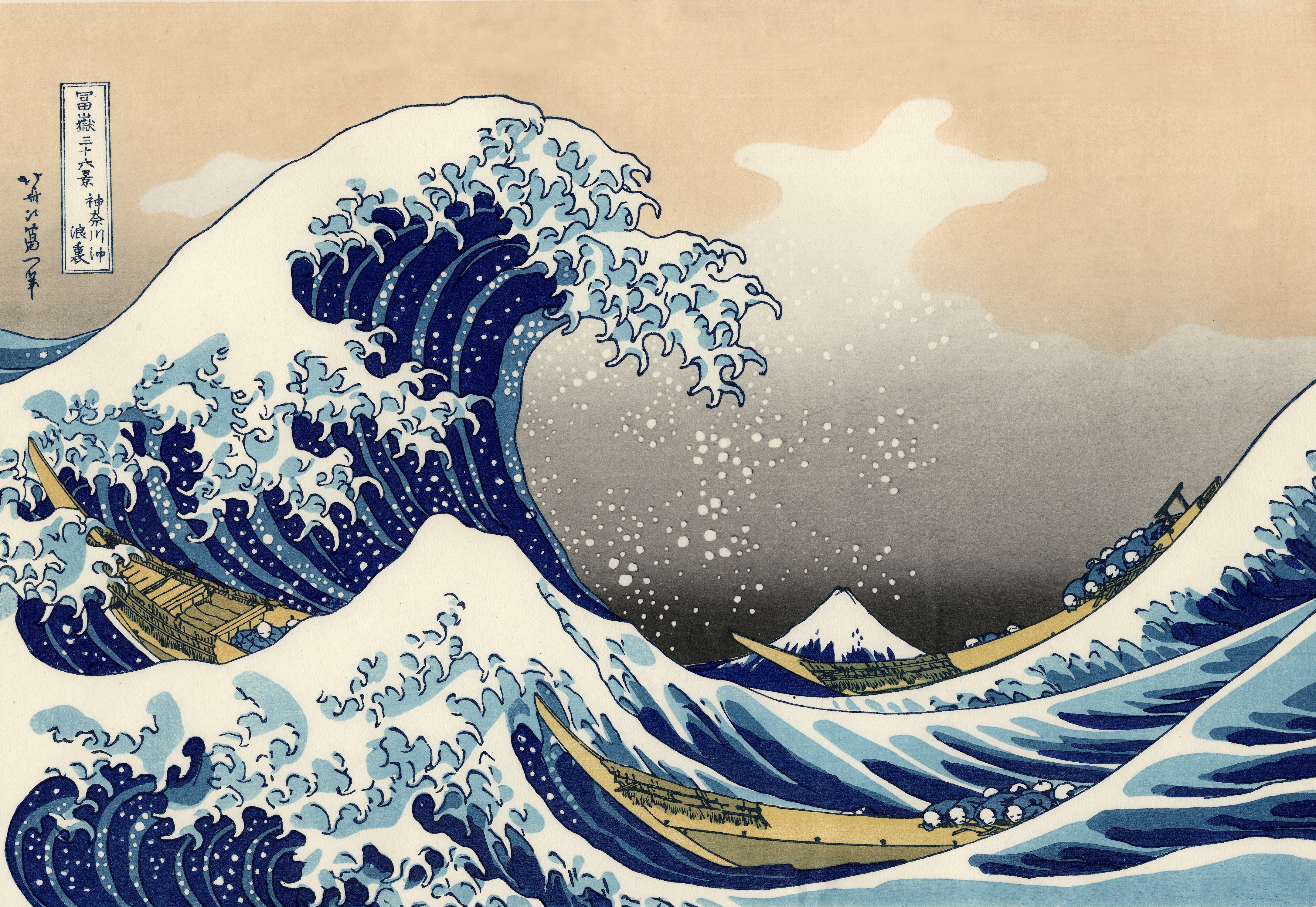
And here’s the style model, Hokusai’s The Great Wave off Kanagawa, which you can download from Wikimedia Commons:
We create a wrapper that loads and preprocesses the input images for us. As we will be working with VGG19, a network that has been trained on ImageNet, we need to transform our input images in the same way that was used training it. Later, we’ll apply the inverse transformation to our combination image before displaying it.
load_and_preprocess_image <- function(path) {
  img <- image_load(path, target_size = img_shape[1:2]) %>%
    image_to_array() %>%
    k_expand_dims(axis = 1) %>%
    imagenet_preprocess_input()
}

deprocess_image <- function(x) {
  x <- x[1, , ,]
  # Remove zero-center by mean pixel
  x[, , 1] <- x[, , 1] + 103.939
  x[, , 2] <- x[, , 2] + 116.779
  x[, , 3] <- x[, , 3] + 123.68
  # 'BGR'->'RGB'
  x <- x[, , c(3, 2, 1)]
  x[x > 255] <- 255
  x[x < 0] <- 0
  x[] <- as.integer(x) / 255
  x
}
Setting the scene
We are going to use a neural network, but we won’t be training it. Neural style transfer is a bit uncommon in that we don’t optimize the network’s weights, but back propagate the loss to the input layer (the image), in order to move it in the desired direction.
We will be interested in two kinds of outputs from the network, corresponding to our two goals. Firstly, we want to keep the combination image similar to the content image, on a high level. In a convnet, upper layers map to more holistic concepts, so we are picking a layer high up in the graph to compare outputs from the source and the combination.
Secondly, the generated image should “look like” the style image. Style corresponds to lower level features like texture, shapes, strokes… So to compare the combination against the style example, we choose a set of lower level conv blocks for comparison and aggregate the results.
content_layers <- c("block5_conv2")
style_layers <- c("block1_conv1",
                 "block2_conv1",
                 "block3_conv1",
                 "block4_conv1",
                 "block5_conv1")

num_content_layers <- length(content_layers)
num_style_layers <- length(style_layers)

get_model <- function() {
  vgg <- application_vgg19(include_top = FALSE, weights = "imagenet")
  vgg$trainable <- FALSE
  style_outputs <- map(style_layers, function(layer) vgg$get_layer(layer)$output)
  content_outputs <- map(content_layers, function(layer) vgg$get_layer(layer)$output)
  model_outputs <- c(style_outputs, content_outputs)
  keras_model(vgg$input, model_outputs)
}
Losses
When optimizing the input image, we will consider three types of losses. Firstly, the content loss: How different is the combination image from the source? Here, we’re using the sum of the squared errors for comparison.
content_loss <- function(content_image, target) {
  k_sum(k_square(target - content_image))
}
Our second concern is having the styles match as closely as possible. Style is commonly operationalized as the Gram matrix of flattened feature maps in a layer. We thus assume that style is related to how maps in a layer correlate with other.
We therefore compute the Gram matrices of the layers we’re interested in (defined above), for the source image as well as the optimization candidate, and compare them, again using the sum of squared errors.
gram_matrix <- function(x) {
  features <- k_batch_flatten(k_permute_dimensions(x, c(3, 1, 2)))
  gram <- k_dot(features, k_transpose(features))
  gram
}

style_loss <- function(gram_target, combination) {
  gram_comb <- gram_matrix(combination)
  k_sum(k_square(gram_target - gram_comb)) /
    (4 * (img_shape[3] ^ 2) * (img_shape[1] * img_shape[2]) ^ 2)
}
Thirdly, we don’t want the combination image to look overly pixelated, thus we’re adding in a regularization component, the total variation in the image:
total_variation_loss <- function(image) {
  y_ij  <- image[1:(img_shape[1] - 1L), 1:(img_shape[2] - 1L),]
  y_i1j <- image[2:(img_shape[1]), 1:(img_shape[2] - 1L),]
  y_ij1 <- image[1:(img_shape[1] - 1L), 2:(img_shape[2]),]
  a <- k_square(y_ij - y_i1j)
  b <- k_square(y_ij - y_ij1)
  k_sum(k_pow(a + b, 1.25))
}
The tricky thing is how to combine these losses. We’ve reached acceptable results with the following weightings, but feel free to play around as you see fit:
content_weight <- 100
style_weight <- 0.8
total_variation_weight <- 0.01
Get model outputs for the content and style images
We need the model’s output for the content and style images, but here it suffices to do this just once. We concatenate both images along the batch dimension, pass that input to the model, and get back a list of outputs, where every element of the list is a 4-d tensor. For the style image, we’re interested in the style outputs at batch position 1, whereas for the content image, we need the content output at batch position 2.
In the below comments, please note that the sizes of dimensions 2 and 3 will differ if you’re loading images at a different size.
get_feature_representations <-
  function(model, content_path, style_path) {

    # dim == (1, 128, 128, 3)
    style_image <-
      load_and_process_image(style_path) %>% k_cast("float32")
    # dim == (1, 128, 128, 3)
    content_image <-
      load_and_process_image(content_path) %>% k_cast("float32")
    # dim == (2, 128, 128, 3)
    stack_images <- k_concatenate(list(style_image, content_image), axis = 1)

    # length(model_outputs) == 6
    # dim(model_outputs[[1]]) = (2, 128, 128, 64)
    # dim(model_outputs[[6]]) = (2, 8, 8, 512)
    model_outputs <- model(stack_images)

    style_features <-
      model_outputs[1:num_style_layers] %>%
      map(function(batch) batch[1, , , ])
    content_features <-
      model_outputs[(num_style_layers + 1):(num_style_layers + num_content_layers)] %>%
      map(function(batch) batch[2, , , ])

    list(style_features, content_features)
  }
Computing the losses
On every iteration, we need to pass the combination image through the model, obtain the style and content outputs, and compute the losses. Again, the code is extensively commented with tensor sizes for easy verification, but please keep in mind that the exact numbers presuppose you’re working with 128x128 images.
compute_loss <-
  function(model, loss_weights, init_image, gram_style_features, content_features) {

    c(style_weight, content_weight) %<-% loss_weights
    model_outputs <- model(init_image)
    style_output_features <- model_outputs[1:num_style_layers]
    content_output_features <-
      model_outputs[(num_style_layers + 1):(num_style_layers + num_content_layers)]

    # style loss
    weight_per_style_layer <- 1 / num_style_layers
    style_score <- 0
    # dim(style_zip[[5]][[1]]) == (512, 512)
    style_zip <- transpose(list(gram_style_features, style_output_features))
    for (l in 1:length(style_zip)) {
      # for l == 1:
      # dim(target_style) == (64, 64)
      # dim(comb_style) == (1, 128, 128, 64)
      c(target_style, comb_style) %<-% style_zip[[l]]
      style_score <- style_score + weight_per_style_layer *
        style_loss(target_style, comb_style[1, , , ])
    }

    # content loss
    weight_per_content_layer <- 1 / num_content_layers
    content_score <- 0
    content_zip <- transpose(list(content_features, content_output_features))
    for (l in 1:length(content_zip)) {
      # dim(comb_content) ==  (1, 8, 8, 512)
      # dim(target_content) == (8, 8, 512)
      c(target_content, comb_content) %<-% content_zip[[l]]
      content_score <- content_score + weight_per_content_layer *
        content_loss(comb_content[1, , , ], target_content)
    }

    # total variation loss
    variation_loss <- total_variation_loss(init_image[1, , ,])

    style_score <- style_score * style_weight
    content_score <- content_score * content_weight
    variation_score <- variation_loss * total_variation_weight

    loss <- style_score + content_score + variation_score
    list(loss, style_score, content_score, variation_score)
  }
Computing the gradients
As soon as we have the losses, obtaining the gradients of the overall loss with respect to the input image is just a matter of calling tape$gradient on the GradientTape. Note that the nested call to compute_loss, and thus the call of the model on our combination image, happens inside the GradientTape context.
compute_grads <-
  function(model, loss_weights, init_image, gram_style_features, content_features) {
    with(tf$GradientTape() %as% tape, {
      scores <-
        compute_loss(model,
                     loss_weights,
                     init_image,
                     gram_style_features,
                     content_features)
    })
    total_loss <- scores[[1]]
    list(tape$gradient(total_loss, init_image), scores)
  }
Training phase
Now it’s time to train! While the natural continuation of this sentence would have been “… the model,” the model we’re training here is not VGG19 (that one we’re just using as a tool), but a minimal setup of just:
- a
Variablethat holds our to-be-optimized image - the loss functions we defined above
- an optimizer that will apply the calculated gradients to the image variable (
tf$train$AdamOptimizer)
Below, we get the style features (of the style image) and the content feature (of the content image) just once, then iterate over the optimization process, saving the output every 100 iterations.
In contrast to the original article and the Deep Learning with R book, but following the Google notebook instead, we’re not using L-BFGS for optimization, but Adam, as our goal here is to provide a concise introduction to eager execution.
However, you could plug in another optimization method if you wanted, replacing
optimizer$apply_gradients(list(tuple(grads, init_image)))
by an algorithm of your choice (and of course, assigning the result of the optimization to the Variable holding the image).
run_style_transfer <- function(content_path, style_path) {
  model <- get_model()
  walk(model$layers, function(layer) layer$trainable = FALSE)

  c(style_features, content_features) %<-%
    get_feature_representations(model, content_path, style_path)
  # dim(gram_style_features[[1]]) == (64, 64)
  gram_style_features <- map(style_features, function(feature) gram_matrix(feature))

  init_image <- load_and_process_image(content_path)
  init_image <- tf$contrib$eager$Variable(init_image, dtype = "float32")

  optimizer <- tf$train$AdamOptimizer(learning_rate = 1,
                                      beta1 = 0.99,
                                      epsilon = 1e-1)

  c(best_loss, best_image) %<-% list(Inf, NULL)
  loss_weights <- list(style_weight, content_weight)

  start_time <- Sys.time()
  global_start <- Sys.time()

  norm_means <- c(103.939, 116.779, 123.68)
  min_vals <- -norm_means
  max_vals <- 255 - norm_means

  for (i in seq_len(num_iterations)) {
    # dim(grads) == (1, 128, 128, 3)
    c(grads, all_losses) %<-% compute_grads(model,
                                            loss_weights,
                                            init_image,
                                            gram_style_features,
                                            content_features)
    c(loss, style_score, content_score, variation_score) %<-% all_losses
    optimizer$apply_gradients(list(tuple(grads, init_image)))
    clipped <- tf$clip_by_value(init_image, min_vals, max_vals)
    init_image$assign(clipped)

    end_time <- Sys.time()

    if (k_cast_to_floatx(loss) < best_loss) {
      best_loss <- k_cast_to_floatx(loss)
      best_image <- init_image
    }

    if (i %% 50 == 0) {
      glue("Iteration: {i}") %>% print()
      glue(
        "Total loss: {k_cast_to_floatx(loss)},
        style loss: {k_cast_to_floatx(style_score)},
        content loss: {k_cast_to_floatx(content_score)},
        total variation loss: {k_cast_to_floatx(variation_score)},
        time for 1 iteration: {(Sys.time() - start_time) %>% round(2)}"
      ) %>% print()

      if (i %% 100 == 0) {
        png(paste0("style_epoch_", i, ".png"))
        plot_image <- best_image$numpy()
        plot_image <- deprocess_image(plot_image)
        plot(as.raster(plot_image), main = glue("Iteration {i}"))
        dev.off()
      }
    }
  }

  glue("Total time: {Sys.time() - global_start} seconds") %>% print()
  list(best_image, best_loss)
}
Ready to run
Now, we’re ready to start the process:
c(best_image, best_loss) %<-% run_style_transfer(content_path, style_path)In our case, results didn’t change much after ~ iteration 1000, and this is how our river landscape was looking:
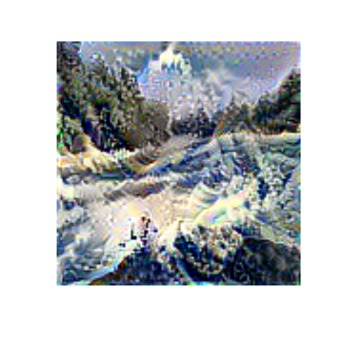
… definitely more inviting than had it been painted by Edvard Munch!
Conclusion
With neural style transfer, some fiddling around may be needed until you get the result you want. But as our example shows, this doesn’t mean the code has to be complicated. Additionally to being easy to grasp, eager execution also lets you add debugging output, and step through the code line-by-line to check on tensor shapes. Until next time in our eager execution series!