As of today, deep learning’s greatest successes have taken place in the realm of supervised learning, requiring lots and lots of annotated training data. However, data does not (normally) come with annotations or labels. Also, unsupervised learning is attractive because of the analogy to human cognition.
On this blog so far, we have seen two major architectures for unsupervised learning: variational autoencoders and generative adversarial networks. Lesser known, but appealing for conceptual as well as for performance reasons are normalizing flows (Jimenez Rezende and Mohamed 2015). In this and the next post, we’ll introduce flows, focusing on how to implement them using TensorFlow Probability (TFP).
In contrast to previous posts involving TFP that accessed its functionality using low-level $-syntax, we now make use of tfprobability, an R wrapper in the style of keras, tensorflow and tfdatasets. A note regarding this package: It is still under heavy development and the API may change. As of this writing, wrappers do not yet exist for all TFP modules, but all TFP functionality is available using $-syntax if need be.
Density estimation and sampling
Back to unsupervised learning, and specifically thinking of variational autoencoders, what are the main things they give us? One thing that’s seldom missing from papers on generative methods are pictures of super-real-looking faces (or bed rooms, or animals …). So evidently sampling (or: generation) is an important part. If we can sample from a model and obtain real-seeming entities, this means the model has learned something about how things are distributed in the world: it has learned a distribution. In the case of variational autoencoders, there is more: The entities are supposed to be determined by a set of distinct, disentangled (hopefully!) latent factors. But this is not the assumption in the case of normalizing flows, so we are not going to elaborate on this here.
As a recap, how do we sample from a VAE? We draw from \(z\), the latent variable, and run the decoder network on it. The result should - we hope - look like it comes from the empirical data distribution. It should not, however, look exactly like any of the items used to train the VAE, or else we have not learned anything useful.
The second thing we may get from a VAE is an assessment of the plausibility of individual data, to be used, for example, in anomaly detection. Here “plausibility” is vague on purpose: With VAE, we don’t have a means to compute an actual density under the posterior.
What if we want, or need, both: generation of samples as well as density estimation? This is where normalizing flows come in.
Normalizing flows
A flow is a sequence of differentiable, invertible mappings from data to a “nice” distribution, something we can easily sample from and use to calculate a density. Let’s take as example the canonical way to generate samples from some distribution, the exponential, say.
We start by asking our random number generator for some number between 0 and 1:1
u <- runif(1)This number we treat as coming from a cumulative probability distribution (CDF) - from an exponential CDF, to be precise. Now that we have a value from the CDF, all we need to do is map that “back” to a value. That mapping CDF -> value we’re looking for is just the inverse of the CDF of an exponential distribution, the CDF being
\[F(x) = 1 - e^{-\lambda x}\]
The inverse then is
\[ F^{-1}(u) = -\frac{1}{\lambda} ln (1 - u) \]
which means we may get our exponential sample doing
lambda <- 0.5 # pick some lambda
x <- -1/lambda * log(1-u)
We see the CDF is actually a flow (or a building block thereof, if we picture most flows as comprising several transformations), since
- It maps data to a uniform distribution between 0 and 1, allowing to assess data likelihood.
- Conversely, it maps a probability to an actual value, thus allowing to generate samples.
From this example, we see why a flow should be invertible, but we don’t yet see why it should be differentiable. This will become clear shortly, but first let’s take a look at how flows are available in tfprobability.
Bijectors
TFP comes with a treasure trove of transformations, called bijectors, ranging from simple computations like exponentiation to more complex ones like the discrete cosine transform.
To get started, let’s use tfprobability to generate samples from the normal distribution.
There is a bijector tfb_normal_cdf() that takes input data to the interval \([0,1]\). Its inverse transform then yields a random variable with the standard normal distribution:
library(tfprobability)
library(tensorflow)
tfe_enable_eager_execution()

library(ggplot2)

b <- tfb_normal_cdf()
u <- runif(1000)
x <- b %>% tfb_inverse(u) %>% as.numeric()

x %>% data.frame(x = .) %>% ggplot(aes(x = x)) + geom_density()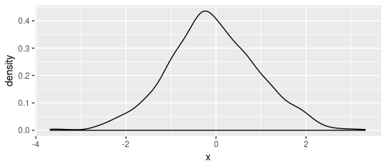
Conversely, we can use this bijector to determine the (log) probability of a sample from the normal distribution. We’ll check against a straightforward use of tfd_normal in the distributions module:
x <- 2.01
d_n <- tfd_normal(loc = 0, scale = 1)

d_n %>% tfd_log_prob(x) %>% as.numeric() # -2.938989
To obtain that same log probability from the bijector, we add two components:
- Firstly, we run the sample through the
forwardtransformation and compute log probability under the uniform distribution. - Secondly, as we’re using the uniform distribution to determine probability of a normal sample, we need to track how probability changes under this transformation. This is done by calling
tfb_forward_log_det_jacobian(to be further elaborated on below).
b <- tfb_normal_cdf()
d_u <- tfd_uniform()

l <- d_u %>% tfd_log_prob(b %>% tfb_forward(x))
j <- b %>% tfb_forward_log_det_jacobian(x, event_ndims = 0)

(l + j) %>% as.numeric() # -2.938989
Why does this work? Let’s get some background.
Probability mass is conserved
Flows are based on the principle that under transformation, probability mass is conserved. Say we have a flow from \(x\) to \(z\): \[z = f(x)\]
Suppose we sample from \(z\) and then, compute the inverse transform to obtain \(x\). We know the probability of \(z\). What is the probability that \(x\), the transformed sample, lies between \(x_0\) and \(x_0 + dx\)?
This probability is \(p(x) \ dx\), the density times the length of the interval. This has to equal the probability that \(z\) lies between \(f(x)\) and \(f(x + dx)\). That new interval has length \(f'(x) dx\), so:
\[p(x) dx = p(z) f'(x) dx\]
Or equivalently
\[p(x) = p(z) * dz/dx\]
Thus, the sample probability \(p(x)\) is determined by the base probability \(p(z)\) of the transformed distribution, multiplied by how much the flow stretches space.
The same goes in higher dimensions: Again, the flow is about the change in probability volume between the \(z\) and \(y\) spaces:
\[p(x) = p(z) \frac{vol(dz)}{vol(dx)}\]
In higher dimensions, the Jacobian replaces the derivative. Then, the change in volume is captured by the absolute value of its determinant:
\[p(\mathbf{x}) = p(f(\mathbf{x})) \ \bigg|det\frac{\partial f({\mathbf{x})}}{\partial{\mathbf{x}}}\bigg|\]
In practice, we work with log probabilities, so
\[log \ p(\mathbf{x}) = log \ p(f(\mathbf{x})) + log \ \bigg|det\frac{\partial f({\mathbf{x})}}{\partial{\mathbf{x}}}\bigg| \]
Let’s see this with another bijector example, tfb_affine_scalar. Below, we construct a mini-flow that maps a few arbitrary chosen \(x\) values to double their value (scale = 2):
x <- c(0, 0.5, 1)
b <- tfb_affine_scalar(shift = 0, scale = 2)
To compare densities under the flow, we choose the normal distribution, and look at the log densities:
d_n <- tfd_normal(loc = 0, scale = 1)
d_n %>% tfd_log_prob(x) %>% as.numeric() # -0.9189385 -1.0439385 -1.4189385
Now apply the flow and compute the new log densities as a sum of the log densities of the corresponding \(x\) values and the log determinant of the Jacobian:
z <- b %>% tfb_forward(x)

(d_n  %>% tfd_log_prob(b %>% tfb_inverse(z))) +
  (b %>% tfb_inverse_log_det_jacobian(z, event_ndims = 0)) %>%
  as.numeric() # -1.6120857 -1.7370857 -2.1120858
We see that as the values get stretched in space (we multiply by 2), the individual log densities go down.
We can verify the cumulative probability stays the same using tfd_transformed_distribution():
d_t <- tfd_transformed_distribution(distribution = d_n, bijector = b)
d_n %>% tfd_cdf(x) %>% as.numeric()  # 0.5000000 0.6914625 0.8413447

d_t %>% tfd_cdf(y) %>% as.numeric()  # 0.5000000 0.6914625 0.8413447
So far, the flows we saw were static - how does this fit into the framework of neural networks?
Training a flow
Given that flows are bidirectional, there are two ways to think about them. Above, we have mostly stressed the inverse mapping: We want a simple distribution we can sample from, and which we can use to compute a density. In that line, flows are sometimes called “mappings from data to noise” - noise mostly being an isotropic Gaussian. However in practice, we don’t have that “noise” yet, we just have data.
So in practice, we have to learn a flow that does such a mapping. We do this by using bijectors with trainable parameters.
We’ll see a very simple example here, and leave “real world flows” to the next post.
The example is based on part 1 of Eric Jang’s introduction to normalizing flows. The main difference (apart from simplification to show the basic pattern) is that we’re using eager execution.
We start from a two-dimensional, isotropic Gaussian, and we want to model data that’s also normal, but with a mean of 1 and a variance of 2 (in both dimensions).
library(tensorflow)
library(tfprobability)

tfe_enable_eager_execution(device_policy = "silent")

library(tfdatasets)

# where we start from
base_dist <- tfd_multivariate_normal_diag(loc = c(0, 0))

# where we want to go
target_dist <- tfd_multivariate_normal_diag(loc = c(1, 1), scale_identity_multiplier = 2)

# create training data from the target distribution
target_samples <- target_dist %>% tfd_sample(1000) %>% tf$cast(tf$float32)

batch_size <- 100
dataset <- tensor_slices_dataset(target_samples) %>%
  dataset_shuffle(buffer_size = dim(target_samples)[1]) %>%
  dataset_batch(batch_size)
Now we’ll build a tiny neural network, consisting of an affine transformation and a nonlinearity.
For the former, we can make use of tfb_affine, the multi-dimensional relative of tfb_affine_scalar.
As to nonlinearities, currently TFP comes with tfb_sigmoid and tfb_tanh, but we can build our own parameterized ReLU using tfb_inline:
# alpha is a learnable parameter
bijector_leaky_relu <- function(alpha) {

  tfb_inline(
    # forward transform leaves positive values untouched and scales negative ones by alpha
    forward_fn = function(x)
      tf$where(tf$greater_equal(x, 0), x, alpha * x),
    # inverse transform leaves positive values untouched and scales negative ones by 1/alpha
    inverse_fn = function(y)
      tf$where(tf$greater_equal(y, 0), y, 1/alpha * y),
    # volume change is 0 when positive and 1/alpha when negative
    inverse_log_det_jacobian_fn = function(y) {
      I <- tf$ones_like(y)
      J_inv <- tf$where(tf$greater_equal(y, 0), I, 1/alpha * I)
      log_abs_det_J_inv <- tf$log(tf$abs(J_inv))
      tf$reduce_sum(log_abs_det_J_inv, axis = 1L)
    },
    forward_min_event_ndims = 1
  )
}
Define the learnable variables for the affine and the PReLU layers:
d <- 2 # dimensionality
r <- 2 # rank of update

# shift of affine bijector
shift <- tf$get_variable("shift", d)
# scale of affine bijector
L <- tf$get_variable('L', c(d * (d + 1) / 2))
# rank-r update
V <- tf$get_variable("V", c(d, r))

# scaling factor of parameterized relu
alpha <- tf$abs(tf$get_variable('alpha', list())) + 0.01
With eager execution, the variables have to be used inside the loss function, so that is where we define the bijectors. Our little flow now is a tfb_chain of bijectors, and we wrap it in a TransformedDistribution (tfd_transformed_distribution) that links source and target distributions.
loss <- function() {

 affine <- tfb_affine(
        scale_tril = tfb_fill_triangular() %>% tfb_forward(L),
        scale_perturb_factor = V,
        shift = shift
      )
 lrelu <- bijector_leaky_relu(alpha = alpha)

 flow <- list(lrelu, affine) %>% tfb_chain()

 dist <- tfd_transformed_distribution(distribution = base_dist,
                          bijector = flow)

 l <- -tf$reduce_mean(dist$log_prob(batch))
 # keep track of progress
 print(round(as.numeric(l), 2))
 l
}
Now we can actually run the training!
optimizer <- tf$train$AdamOptimizer(1e-4)

n_epochs <- 100
for (i in 1:n_epochs) {
  iter <- make_iterator_one_shot(dataset)
  until_out_of_range({
    batch <- iterator_get_next(iter)
    optimizer$minimize(loss)
  })
}
Outcomes will differ depending on random initialization, but you should see a steady (if slow) progress. Using bijectors, we have actually trained and defined a little neural network.
Outlook
Undoubtedly, this flow is too simple to model complex data, but it’s instructive to have seen the basic principles before delving into more complex flows. In the next post, we’ll check out autoregressive flows, again using TFP and tfprobability.
Yes, using
runif(). Just imagine there were no correspondingrexp()in R…↩︎