In a previous post, we showed how to use tfprobability – the R interface to TensorFlow Probability – to build a multilevel, or partial pooling model of tadpole survival in differently sized (and thus, differing in inhabitant number) tanks.
A completely pooled model would have resulted in a global estimate of survival count, irrespective of tank, while an unpooled model would have learned to predict survival count for each tank separately. The former approach does not take into account different circumstances; the latter does not make use of common information. (Also, it clearly has no predictive use unless we want to make predictions for the very same entities we used to train the model.)
In contrast, a partially pooled model lets you make predictions for the familiar, as well as new entities: Just use the appropriate prior.
Assuming we are in fact interested in the same entities – why would we want to apply partial pooling? For the same reasons so much effort in machine learning goes into devising regularization mechanisms. We don’t want to overfit too much to actual measurements, be they related to the same entity or a class of entities. If I want to predict my heart rate as I wake up next morning, based on a single measurement I’m taking now (let’s say it’s evening and I’m frantically typing a blog post), I better take into account some facts about heart rate behavior in general (instead of just projecting into the future the exact value measured right now).
In the tadpole example, this means we expect generalization to work better for tanks with many inhabitants, compared to more solitary environments. For the latter ones, we better take a peek at survival rates from other tanks, to supplement the sparse, idiosyncratic information available. Or using the technical term, in the latter case we hope for the model to shrink its estimates toward the overall mean more noticeably than in the former.
This type of information sharing is already very useful, but it gets better. The tadpole model is a varying intercepts model, as McElreath calls it (or random intercepts, as it is sometimes – confusingly – called 1) – intercepts referring to the way we make predictions for entities (here: tanks), with no predictor variables present. So if we can pool information about intercepts, why not pool information about slopes as well? This will allow us to, in addition, make use of relationships between variables learnt on different entities in the training set.
So as you might have guessed by now, varying slopes (or random slopes, if you will) is the topic of today’s post. Again, we take up an example from McElreath’s book, and show how to accomplish the same thing with tfprobability.
Coffee, please
Unlike the tadpole case, this time we work with simulated data. This is the data McElreath uses to introduce the varying slopes modeling technique; he then goes on and applies it to one of the book’s most featured datasets, the pro-social (or indifferent, rather!) chimpanzees. For today, we stay with the simulated data for two reasons: First, the subject matter per se is non-trivial enough; and second, we want to keep careful track of what our model does, and whether its output is sufficiently close to the results McElreath obtained from Stan 2.
So, the scenario is this. 3 Cafés vary in how popular they are. In a popular café, when you order coffee, you’re likely to wait. In a less popular café, you’ll likely be served much faster. That’s one thing. Second, all cafés tend to be more crowded in the mornings than in the afternoons. Thus in the morning, you’ll wait longer than in the afternoon – this goes for the popular as well as the less popular cafés.
In terms of intercepts and slopes, we can picture the morning waits as intercepts, and the resultant afternoon waits as arising due to the slopes of the lines joining each morning and afternoon wait, respectively.
So when we partially-pool intercepts, we have one “intercept prior” (itself constrained by a prior, of course), and a set of café-specific intercepts that will vary around it. When we partially-pool slopes, we have a “slope prior” reflecting the overall relationship between morning and afternoon waits, and a set of café-specific slopes reflecting the individual relationships. Cognitively, that means that if you have never been to the Café Gerbeaud in Budapest but have been to cafés before, you might have a less-than-uninformed idea about how long you are going to wait; it also means that if you normally get your coffee in your favorite corner café in the mornings, and now you pass by there in the afternoon, you have an approximate idea how long it’s going to take (namely, fewer minutes than in the mornings).
So is that all? Actually, no. In our scenario, intercepts and slopes are related. If, at a less popular café, I always get my coffee before two minutes have passed, there is little room for improvement. At a highly popular café though, if it could easily take ten minutes in the mornings, then there is quite some potential for decrease in waiting time in the afternoon. So in my prediction for this afternoon’s waiting time, I should factor in this interaction effect.
So, now that we have an idea of what this is all about, let’s see how we can model these effects with tfprobability. But first, we actually have to generate the data.
Simulate the data
We directly follow McElreath in the way the data are generated.
##### Inputs needed to generate the covariance matrix between intercepts and slopes #####

# average morning wait time
a <- 3.5
# average difference afternoon wait time
# we wait less in the afternoons
b <- -1
# standard deviation in the (café-specific) intercepts
sigma_a <- 1
# standard deviation in the (café-specific) slopes
sigma_b <- 0.5
# correlation between intercepts and slopes
# the higher the intercept, the more the wait goes down
rho <- -0.7


##### Generate the covariance matrix #####

# means of intercepts and slopes
mu <- c(a, b)
# standard deviations of means and slopes
sigmas <- c(sigma_a, sigma_b)
# correlation matrix
# a correlation matrix has ones on the diagonal and the correlation in the off-diagonals
rho <- matrix(c(1, rho, rho, 1), nrow = 2)
# now matrix multiply to get covariance matrix
cov_matrix <- diag(sigmas) %*% rho %*% diag(sigmas)


##### Generate the café-specific intercepts and slopes #####

# 20 cafés overall
n_cafes <- 20

library(MASS)
set.seed(5) # used to replicate example
# multivariate distribution of intercepts and slopes
vary_effects <- mvrnorm(n_cafes , mu ,cov_matrix)
# intercepts are in the first column
a_cafe <- vary_effects[ ,1]
# slopes are in the second
b_cafe <- vary_effects[ ,2]


##### Generate the actual wait times #####

set.seed(22)
# 10 visits per café
n_visits <- 10

# alternate values for mornings and afternoons in the data frame
afternoon <- rep(0:1, n_visits * n_cafes/2)
# data for each café are consecutive rows in the data frame
cafe_id <- rep(1:n_cafes, each = n_visits)

# the regression equation for the mean waiting time
mu <- a_cafe[cafe_id] + b_cafe[cafe_id] * afternoon
# standard deviation of waiting time within cafés
sigma <- 0.5 # std dev within cafes
# generate instances of waiting times
wait <- rnorm(n_visits * n_cafes, mu, sigma)

d <- data.frame(cafe = cafe_id, afternoon = afternoon, wait = wait)
Take a glimpse at the data:
d %>% glimpse()Observations: 200
Variables: 3
$ cafe <int> 1, 1, 1, 1, 1, 1, 1, 1, 1, 1, 2, 2, 2, 2, 2, 2, 2, 2, 2, 2, 3,...
$ afternoon <int> 0, 1, 0, 1, 0, 1, 0, 1, 0, 1, 0, 1, 0, 1, 0, 1, 0, 1, 0, 1, 0,...
$ wait <dbl> 3.9678929, 3.8571978, 4.7278755, 2.7610133, 4.1194827, 3.54365,...On to building the model.
The model
As in the previous post on multi-level modeling, we use tfd_joint_distribution_sequential to define the model and Hamiltonian Monte Carlo for sampling. Consider taking a look at the first section of that post for a quick reminder of the overall procedure.
Before we code the model, let’s quickly get library loading out of the way. Importantly, again just like in the previous post, we need to install a master build of TensorFlow Probability, as we’re making use of very new features not yet available in the current release version. The same goes for the R packages tensorflow and tfprobability: Please install the respective development versions from github.
devtools::install_github("rstudio/tensorflow")
devtools::install_github("rstudio/tfprobability")

# this will install the latest nightlies of TensorFlow as well as TensorFlow Probability
tensorflow::install_tensorflow(version = "nightly")

library(tensorflow)
tf$compat$v1$enable_v2_behavior()

library(tfprobability)

library(tidyverse)
library(zeallot)
library(abind)
library(gridExtra)
library(HDInterval)
library(ellipse)
Now here is the model definition. We’ll go through it step by step in an instant.
model <- function(cafe_id) {
  tfd_joint_distribution_sequential(
      list(
        # rho, the prior for the correlation matrix between intercepts and slopes
        tfd_cholesky_lkj(2, 2),
        # sigma, prior variance for the waiting time
        tfd_sample_distribution(tfd_exponential(rate = 1), sample_shape = 1),
        # sigma_cafe, prior of variances for intercepts and slopes (vector of 2)
        tfd_sample_distribution(tfd_exponential(rate = 1), sample_shape = 2),
        # b, the prior mean for the slopes
        tfd_sample_distribution(tfd_normal(loc = -1, scale = 0.5), sample_shape = 1),
        # a, the prior mean for the intercepts
        tfd_sample_distribution(tfd_normal(loc = 5, scale = 2), sample_shape = 1),
        # mvn, multivariate distribution of intercepts and slopes
        # shape: batch size, 20, 2
        function(a,b,sigma_cafe,sigma,chol_rho)
          tfd_sample_distribution(
            tfd_multivariate_normal_tri_l(
              loc = tf$concat(list(a,b), axis = -1L),
              scale_tril = tf$linalg$LinearOperatorDiag(sigma_cafe)$matmul(chol_rho)),
            sample_shape = n_cafes),
        # waiting time
        # shape should be batch size, 200
        function(mvn, a, b, sigma_cafe, sigma)
          tfd_independent(
            # need to pull out the correct cafe_id in the middle column
            tfd_normal(
              loc = (tf$gather(mvn[ , , 1], cafe_id, axis = -1L) +
                       tf$gather(mvn[ , , 2], cafe_id, axis = -1L) * afternoon),
              scale=sigma),  # Shape [batch,  1]
        reinterpreted_batch_ndims=1
        )
    )
  )
}
The first five distributions are priors. First, we have the prior for the correlation matrix.
Basically, this would be an LKJ distribution of shape 2x2 and with concentration parameter equal to 2.
For performance reasons, we work with a version that inputs and outputs Cholesky factors instead:
# rho, the prior correlation matrix between intercepts and slopes
tfd_cholesky_lkj(2, 2)
What kind of prior is this? As McElreath keeps reminding us, nothing is more instructive than sampling from the prior. For us to see what’s going on, we use the base LKJ distribution, not the Cholesky one:
corr_prior <- tfd_lkj(2, 2)
correlation <- (corr_prior %>% tfd_sample(100))[ , 1, 2] %>% as.numeric()
library(ggplot2)
data.frame(correlation) %>% ggplot(aes(x = correlation)) + geom_density()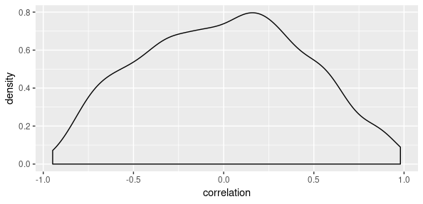
So this prior is moderately skeptical about strong correlations, but pretty open to learning from data.
The next distribution in line
# sigma, prior variance for the waiting time
tfd_sample_distribution(tfd_exponential(rate = 1), sample_shape = 1)
is the prior for the variance of the waiting time, the very last distribution in the list.
Next is the prior distribution of variances for the intercepts and slopes. This prior is the same for both cases, but we specify a sample_shape of 2 to get two individual samples.
# sigma_cafe, prior of variances for intercepts and slopes (vector of 2)
tfd_sample_distribution(tfd_exponential(rate = 1), sample_shape = 2)
Now that we have the respective prior variances, we move on to the prior means. Both are normal distributions.
# b, the prior mean for the slopes
tfd_sample_distribution(tfd_normal(loc = -1, scale = 0.5), sample_shape = 1)
# a, the prior mean for the intercepts
tfd_sample_distribution(tfd_normal(loc = 5, scale = 2), sample_shape = 1)On to the heart of the model, where the partial pooling happens. We are going to construct partially-pooled intercepts and slopes for all of the cafés. Like we said above, intercepts and slopes are not independent; they interact. Thus, we need to use a multivariate normal distribution. The means are given by the prior means defined right above, while the covariance matrix is built from the above prior variances and the prior correlation matrix. The output shape here is determined by the number of cafés: We want an intercept and a slope for every café.
# mvn, multivariate distribution of intercepts and slopes
# shape: batch size, 20, 2
function(a,b,sigma_cafe,sigma,chol_rho)
  tfd_sample_distribution(
    tfd_multivariate_normal_tri_l(
      loc = tf$concat(list(a,b), axis = -1L),
      scale_tril = tf$linalg$LinearOperatorDiag(sigma_cafe)$matmul(chol_rho)),
  sample_shape = n_cafes)
Finally, we sample the actual waiting times. This code pulls out the correct intercepts and slopes from the multivariate normal and outputs the mean waiting time, dependent on what café we’re in and whether it’s morning or afternoon.
        # waiting time
        # shape: batch size, 200
        function(mvn, a, b, sigma_cafe, sigma)
          tfd_independent(
            # need to pull out the correct cafe_id in the middle column
            tfd_normal(
              loc = (tf$gather(mvn[ , , 1], cafe_id, axis = -1L) +
                       tf$gather(mvn[ , , 2], cafe_id, axis = -1L) * afternoon),
              scale=sigma),
        reinterpreted_batch_ndims=1
        )
Before running the sampling, it’s always a good idea to do a quick check on the model.
n_cafes <- 20
cafe_id <- tf$cast((d$cafe - 1) %% 20, tf$int64)

afternoon <- d$afternoon
wait <- d$wait
We sample from the model and then, check the log probability.
m <- model(cafe_id)

s <- m %>% tfd_sample(3)
m %>% tfd_log_prob(s)
We want a scalar log probability per member in the batch, which is what we get.
tf.Tensor([-466.1392 -149.92587 -196.51688], shape=(3,), dtype=float32)Running the chains
The actual Monte Carlo sampling works just like in the previous post, with one exception. Sampling happens in unconstrained parameter space, but at the end we need to get valid correlation matrix parameters rho and valid variances sigma and sigma_cafe. Conversion between spaces is done via TFP bijectors. Luckily, this is not something we have to do as users; all we need to specify are appropriate bijectors. For the normal distributions in the model, there is nothing to do.
constraining_bijectors <- list(
  # make sure the rho[1:4] parameters are valid for a Cholesky factor
  tfb_correlation_cholesky(),
  # make sure variance is positive
  tfb_exp(),
  # make sure variance is positive
  tfb_exp(),
  tfb_identity(),
  tfb_identity(),
  tfb_identity()
)
Now we can set up the Hamiltonian Monte Carlo sampler.
n_steps <- 500
n_burnin <- 500
n_chains <- 4

# set up the optimization objective
logprob <- function(rho, sigma, sigma_cafe, b, a, mvn)
  m %>% tfd_log_prob(list(rho, sigma, sigma_cafe, b, a, mvn, wait))

# initial states for the sampling procedure
c(initial_rho, initial_sigma, initial_sigma_cafe, initial_b, initial_a, initial_mvn, .) %<-%
  (m %>% tfd_sample(n_chains))

# HMC sampler, with the above bijectors and step size adaptation
hmc <- mcmc_hamiltonian_monte_carlo(
  target_log_prob_fn = logprob,
  num_leapfrog_steps = 3,
  step_size = list(0.1, 0.1, 0.1, 0.1, 0.1, 0.1)
) %>%
  mcmc_transformed_transition_kernel(bijector = constraining_bijectors) %>%
  mcmc_simple_step_size_adaptation(target_accept_prob = 0.8,
                                   num_adaptation_steps = n_burnin)
Again, we can obtain additional diagnostics (here: step sizes and acceptance rates) by registering a trace function:
trace_fn <- function(state, pkr) {
  list(pkr$inner_results$inner_results$is_accepted,
       pkr$inner_results$inner_results$accepted_results$step_size)
}
Here, then, is the sampling function. Note how we use tf_function to put it on the graph. At least as of today, this makes a huge difference in sampling performance when using eager execution.
run_mcmc <- function(kernel) {
  kernel %>% mcmc_sample_chain(
    num_results = n_steps,
    num_burnin_steps = n_burnin,
    current_state = list(initial_rho,
                         tf$ones_like(initial_sigma),
                         tf$ones_like(initial_sigma_cafe),
                         initial_b,
                         initial_a,
                         initial_mvn),
    trace_fn = trace_fn
  )
}

run_mcmc <- tf_function(run_mcmc)
res <- hmc %>% run_mcmc()

mcmc_trace <- res$all_states
So how do our samples look, and what do we get in terms of posteriors? Let’s see.
Results
At this moment, mcmc_trace is a list of tensors of different shapes, dependent on how we defined the parameters. We need to do a bit of post-processing to be able to summarise and display the results.
# the actual mcmc samples
# for the trace plots, we want to have them in shape (500, 4, 49)
# that is: (number of steps, number of chains, number of parameters)
samples <- abind(
  # rho 1:4
  as.array(mcmc_trace[[1]] %>% tf$reshape(list(tf$cast(n_steps, tf$int32), tf$cast(n_chains, tf$int32), 4L))),
  # sigma
  as.array(mcmc_trace[[2]]),
  # sigma_cafe 1:2
  as.array(mcmc_trace[[3]][ , , 1]),
  as.array(mcmc_trace[[3]][ , , 2]),
  # b
  as.array(mcmc_trace[[4]]),
  # a
  as.array(mcmc_trace[[5]]),
  # mvn 10:49
  as.array( mcmc_trace[[6]] %>% tf$reshape(list(tf$cast(n_steps, tf$int32), tf$cast(n_chains, tf$int32), 40L))),
  along = 3)

# the effective sample sizes
# we want them in shape (4, 49), which is (number of chains * number of parameters)
ess <- mcmc_effective_sample_size(mcmc_trace)
ess <- cbind(
  # rho 1:4
  as.matrix(ess[[1]] %>% tf$reshape(list(tf$cast(n_chains, tf$int32), 4L))),
  # sigma
  as.matrix(ess[[2]]),
  # sigma_cafe 1:2
  as.matrix(ess[[3]][ , 1, drop = FALSE]),
  as.matrix(ess[[3]][ , 2, drop = FALSE]),
  # b
  as.matrix(ess[[4]]),
  # a
  as.matrix(ess[[5]]),
  # mvn 10:49
  as.matrix(ess[[6]] %>% tf$reshape(list(tf$cast(n_chains, tf$int32), 40L)))
  )

# the rhat values
# we want them in shape (49), which is (number of parameters)
rhat <- mcmc_potential_scale_reduction(mcmc_trace)
rhat <- c(
  # rho 1:4
  as.double(rhat[[1]] %>% tf$reshape(list(4L))),
  # sigma
  as.double(rhat[[2]]),
  # sigma_cafe 1:2
  as.double(rhat[[3]][1]),
  as.double(rhat[[3]][2]),
  # b
  as.double(rhat[[4]]),
  # a
  as.double(rhat[[5]]),
  # mvn 10:49
  as.double(rhat[[6]] %>% tf$reshape(list(40L)))
  )
Trace plots
How well do the chains mix?
prep_tibble <- function(samples) {
  as_tibble(samples, .name_repair = ~ c("chain_1", "chain_2", "chain_3", "chain_4")) %>%
    add_column(sample = 1:n_steps) %>%
    gather(key = "chain", value = "value", -sample)
}

plot_trace <- function(samples) {
  prep_tibble(samples) %>%
    ggplot(aes(x = sample, y = value, color = chain)) +
    geom_line() +
    theme_light() +
    theme(legend.position = "none",
          axis.title = element_blank(),
          axis.text = element_blank(),
          axis.ticks = element_blank())
}

plot_traces <- function(sample_array, num_params) {
  plots <- purrr::map(1:num_params, ~ plot_trace(sample_array[ , , .x]))
  do.call(grid.arrange, plots)
}

plot_traces(samples, 49)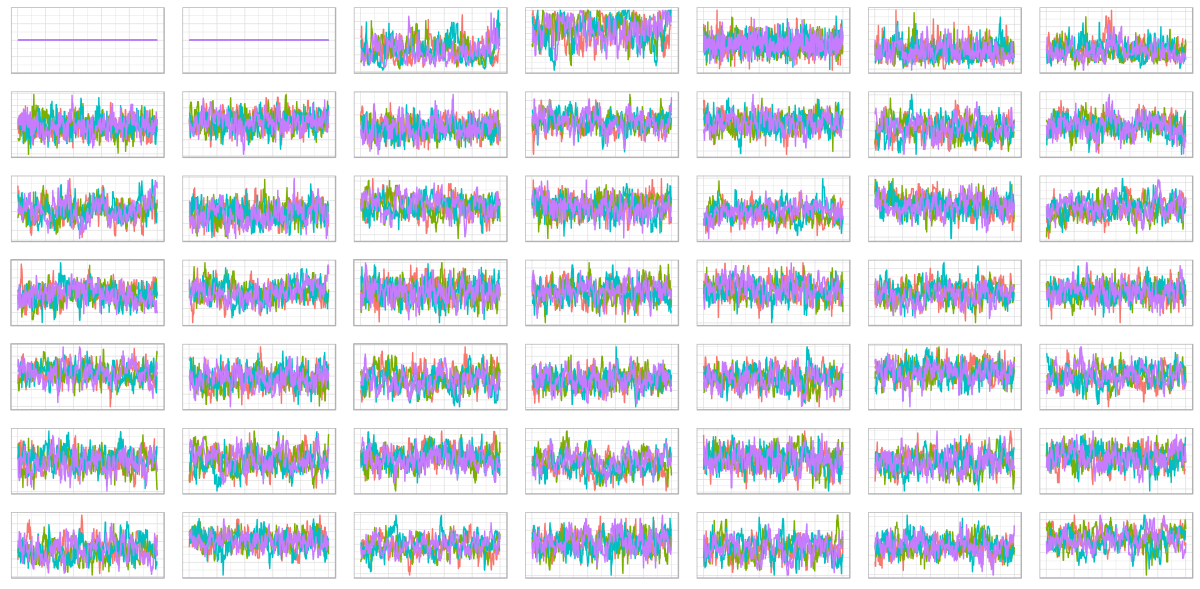
Awesome! (The first two parameters of rho, the Cholesky factor of the correlation matrix, need to stay fixed at 1 and 0, respectively.)
Now, on to some summary statistics on the posteriors of the parameters.
Parameters
Like last time, we display posterior means and standard deviations, as well as the highest posterior density interval (HPDI). We add effective sample sizes and rhat values.
column_names <- c(
  paste0("rho_", 1:4),
  "sigma",
  paste0("sigma_cafe_", 1:2),
  "b",
  "a",
  c(rbind(paste0("a_cafe_", 1:20), paste0("b_cafe_", 1:20)))
)

all_samples <- matrix(samples, nrow = n_steps * n_chains, ncol = 49)
all_samples <- all_samples %>%
  as_tibble(.name_repair = ~ column_names)

all_samples %>% glimpse()

means <- all_samples %>%
  summarise_all(list (mean)) %>%
  gather(key = "key", value = "mean")

sds <- all_samples %>%
  summarise_all(list (sd)) %>%
  gather(key = "key", value = "sd")

hpdis <-
  all_samples %>%
  summarise_all(list(~ list(hdi(.) %>% t() %>% as_tibble()))) %>%
   unnest()

 hpdis_lower <- hpdis %>% select(-contains("upper")) %>%
   rename(lower0 = lower) %>%
   gather(key = "key", value = "lower") %>%
   arrange(as.integer(str_sub(key, 6))) %>%
   mutate(key = column_names)

 hpdis_upper <- hpdis %>% select(-contains("lower")) %>%
   rename(upper0 = upper) %>%
   gather(key = "key", value = "upper") %>%
   arrange(as.integer(str_sub(key, 6))) %>%
   mutate(key = column_names)

summary <- means %>%
  inner_join(sds, by = "key") %>%
  inner_join(hpdis_lower, by = "key") %>%
  inner_join(hpdis_upper, by = "key")

ess <- apply(ess, 2, mean)

summary_with_diag <- summary %>% add_column(ess = ess, rhat = rhat)
print(summary_with_diag, n = 49)
# A tibble: 49 x 7
key mean sd lower upper ess rhat
<chr> <dbl> <dbl> <dbl> <dbl> <dbl> <dbl>
1 rho_1 1 0 1 1 NaN NaN
2 rho_2 0 0 0 0 NaN NaN
3 rho_3 -0.517 0.176 -0.831 -0.195 42.4 1.01
4 rho_4 0.832 0.103 0.644 1.000 46.5 1.02
5 sigma 0.473 0.0264 0.420 0.523 424. 1.00
6 sigma_cafe_1 0.967 0.163 0.694 1.29 97.9 1.00
7 sigma_cafe_2 0.607 0.129 0.386 0.861 42.3 1.03
8 b -1.14 0.141 -1.43 -0.864 95.1 1.00
9 a 3.66 0.218 3.22 4.07 75.3 1.01
10 a_cafe_1 4.20 0.192 3.83 4.57 83.9 1.01
11 b_cafe_1 -1.13 0.251 -1.63 -0.664 63.6 1.02
12 a_cafe_2 2.17 0.195 1.79 2.54 59.3 1.01
13 b_cafe_2 -0.923 0.260 -1.42 -0.388 46.0 1.01
14 a_cafe_3 4.40 0.195 4.02 4.79 56.7 1.01
15 b_cafe_3 -1.97 0.258 -2.52 -1.51 43.9 1.01
16 a_cafe_4 3.22 0.199 2.80 3.57 58.7 1.02
17 b_cafe_4 -1.20 0.254 -1.70 -0.713 36.3 1.01
18 a_cafe_5 1.86 0.197 1.45 2.20 52.8 1.03
19 b_cafe_5 -0.113 0.263 -0.615 0.390 34.6 1.04
20 a_cafe_6 4.26 0.210 3.87 4.67 43.4 1.02
21 b_cafe_6 -1.30 0.277 -1.80 -0.713 41.4 1.05
22 a_cafe_7 3.61 0.198 3.23 3.98 44.9 1.01
23 b_cafe_7 -1.02 0.263 -1.51 -0.489 37.7 1.03
24 a_cafe_8 3.95 0.189 3.59 4.31 73.1 1.01
25 b_cafe_8 -1.64 0.248 -2.10 -1.13 60.7 1.02
26 a_cafe_9 3.98 0.212 3.57 4.37 76.3 1.03
27 b_cafe_9 -1.29 0.273 -1.83 -0.776 57.8 1.05
28 a_cafe_10 3.60 0.187 3.24 3.96 104. 1.01
29 b_cafe_10 -1.00 0.245 -1.47 -0.512 70.4 1.00
30 a_cafe_11 1.95 0.200 1.56 2.35 55.9 1.03
31 b_cafe_11 -0.449 0.266 -1.00 0.0619 42.5 1.04
32 a_cafe_12 3.84 0.195 3.46 4.22 76.0 1.02
33 b_cafe_12 -1.17 0.259 -1.65 -0.670 62.5 1.03
34 a_cafe_13 3.88 0.201 3.50 4.29 62.2 1.02
35 b_cafe_13 -1.81 0.270 -2.30 -1.29 48.3 1.03
36 a_cafe_14 3.19 0.212 2.82 3.61 65.9 1.07
37 b_cafe_14 -0.961 0.278 -1.49 -0.401 49.9 1.06
38 a_cafe_15 4.46 0.212 4.08 4.91 62.0 1.09
39 b_cafe_15 -2.20 0.290 -2.72 -1.59 47.8 1.11
40 a_cafe_16 3.41 0.193 3.02 3.78 62.7 1.02
41 b_cafe_16 -1.07 0.253 -1.54 -0.567 48.5 1.05
42 a_cafe_17 4.22 0.201 3.82 4.60 58.7 1.01
43 b_cafe_17 -1.24 0.273 -1.74 -0.703 43.8 1.01
44 a_cafe_18 5.77 0.210 5.34 6.18 66.0 1.02
45 b_cafe_18 -1.05 0.284 -1.61 -0.511 49.8 1.02
46 a_cafe_19 3.23 0.203 2.88 3.65 52.7 1.02
47 b_cafe_19 -0.232 0.276 -0.808 0.243 45.2 1.01
48 a_cafe_20 3.74 0.212 3.35 4.21 48.2 1.04
49 b_cafe_20 -1.09 0.281 -1.58 -0.506 36.5 1.05So what do we have? If you run this “live”, for the rows a_cafe_n resp. b_cafe_n, you see a nice alternation of white and red coloring: For all cafés, the inferred slopes are negative.
The inferred slope prior (b) is around -1.14, which is not too far off from the value we used for sampling: 1.
The rho posterior estimates, admittedly, are less useful unless you are accustomed to compose Cholesky factors in your head. We compute the resulting posterior correlations and their mean:
-0.5166775The value we used for sampling was -0.7, so we see the regularization effect. In case you’re wondering, for the same data Stan yields an estimate of -0.5.
Finally, let’s display equivalents to McElreath’s figures illustrating shrinkage on the parameter (café-specific intercepts and slopes) as well as the outcome (morning resp. afternoon waiting times) scales.
Shrinkage
As expected, we see that the individual intercepts and slopes are pulled towards the mean – the more, the further away they are from the center.
# just like McElreath, compute unpooled estimates directly from data
a_empirical <- d %>%
  filter(afternoon == 0) %>%
  group_by(cafe) %>%
  summarise(a = mean(wait)) %>%
  select(a)

b_empirical <- d %>%
  filter(afternoon == 1) %>%
  group_by(cafe) %>%
  summarise(b = mean(wait)) %>%
  select(b) -
  a_empirical

empirical_estimates <- bind_cols(
  a_empirical,
  b_empirical,
  type = rep("data", 20))

posterior_estimates <- tibble(
  a = means %>% filter(
  str_detect(key, "^a_cafe")) %>% select(mean) %>% pull(),
  b = means %>% filter(
    str_detect(key, "^b_cafe")) %>% select(mean)  %>% pull(),
  type = rep("posterior", 20))

all_estimates <- bind_rows(empirical_estimates, posterior_estimates)

# compute posterior mean bivariate Gaussian
# again following McElreath
mu_est <- c(means[means$key == "a", 2], means[means$key == "b", 2]) %>% unlist()
rho_est <- mean_rho
sa_est <- means[means$key == "sigma_cafe_1", 2] %>% unlist()
sb_est <- means[means$key == "sigma_cafe_2", 2] %>% unlist()
cov_ab <- sa_est * sb_est * rho_est
sigma_est <- matrix(c(sa_est^2, cov_ab, cov_ab, sb_est^2), ncol=2)

alpha_levels <- c(0.1, 0.3, 0.5, 0.8, 0.99)
names(alpha_levels) <- alpha_levels

contour_data <- plyr::ldply(
  alpha_levels,
  ellipse,
  x = sigma_est,
  scale = c(1, 1),
  centre = mu_est
)

ggplot() +
  geom_point(data = all_estimates, mapping = aes(x = a, y = b, color = type)) +
  geom_path(data = contour_data, mapping = aes(x = x, y = y, group = .id))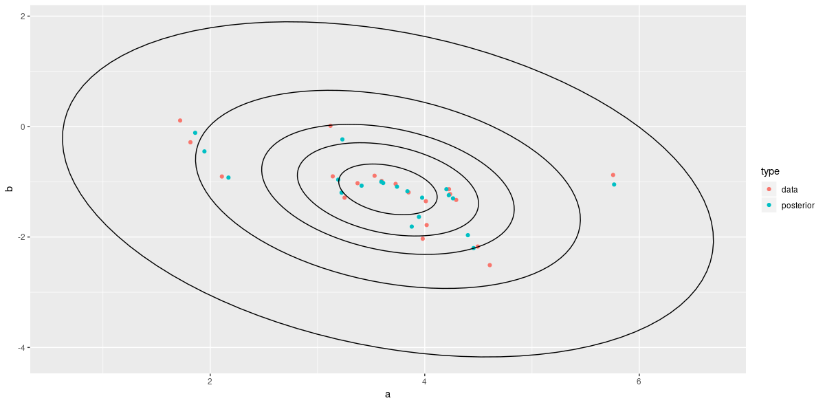
The same behavior is visible on the outcome scale.
wait_times  <- all_estimates %>%
  mutate(morning = a, afternoon = a + b)

# simulate from posterior means
v <- MASS::mvrnorm(1e4 , mu_est , sigma_est)
v[ ,2] <- v[ ,1] + v[ ,2] # calculate afternoon wait
# construct empirical covariance matrix
sigma_est2 <- cov(v)
mu_est2 <- mu_est
mu_est2[2] <- mu_est[1] + mu_est[2]

contour_data <- plyr::ldply(
  alpha_levels,
  ellipse,
  x = sigma_est2 %>% unname(),
  scale = c(1, 1),
  centre = mu_est2
)

ggplot() +
  geom_point(data = wait_times, mapping = aes(x = morning, y = afternoon, color = type)) +
  geom_path(data = contour_data, mapping = aes(x = x, y = y, group = .id))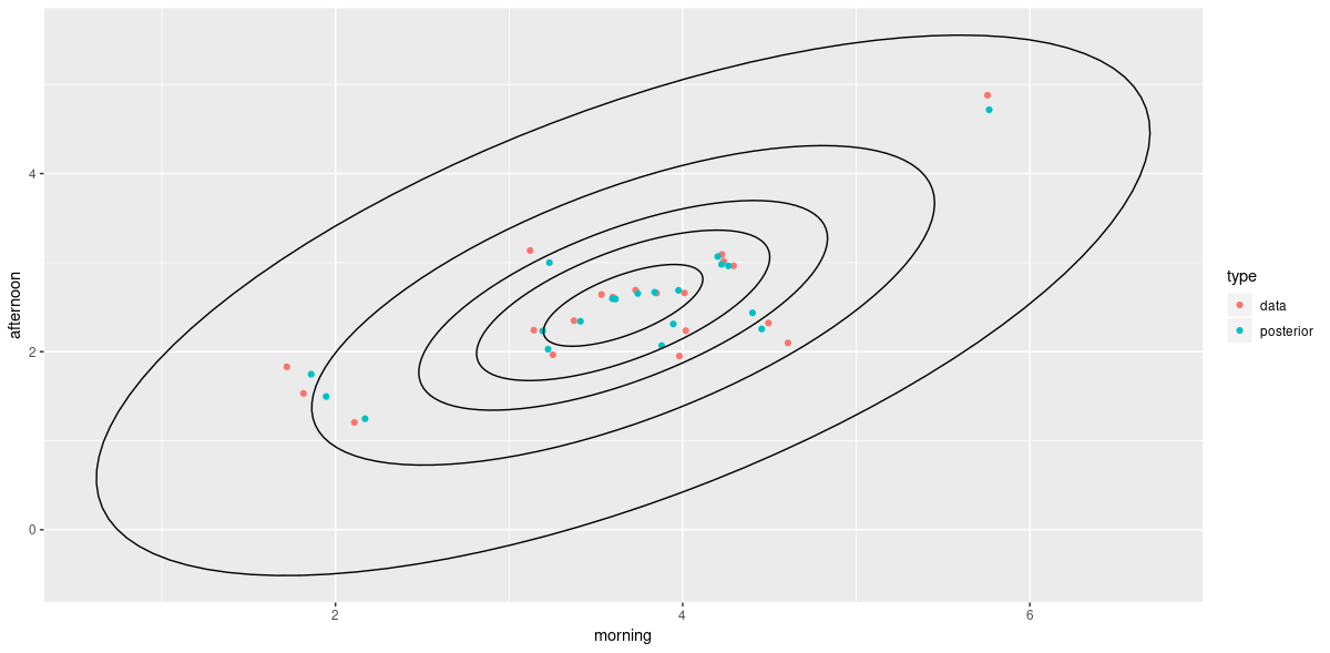
Wrapping up
By now, we hope we have convinced you of the power inherent in Bayesian modeling, as well as conveyed some ideas on how this is achievable with TensorFlow Probability. As with every DSL though, it takes time to proceed from understanding worked examples to design your own models. And not just time – it helps to have seen a lot of different models, focusing on different tasks and applications. On this blog, we plan to loosely follow up on Bayesian modeling with TFP, picking up some of the tasks and challenges elaborated on in the later chapters of McElreath’s book. Thanks for reading!
cf. the Wikipedia article on multilevel models for a collection of terms encountered when dealing with this subject, and e.g. Gelman’s dissection of various ways random effects are defined↩︎
We won’t overload this post by explicitly comparing results here, but we did that when writing the code.↩︎
Disclaimer: We have not verified whether this is an adequate model of the world, but it really doesn’t matter either.↩︎