About six months ago, we showed how to create a custom wrapper to obtain uncertainty estimates from a Keras network. Today we present a less laborious, as well faster-running way using tfprobability, the R wrapper to TensorFlow Probability. Like most posts on this blog, this one won’t be short, so let’s quickly state what you can expect in return of reading time.
What to expect from this post
Starting from what not to expect: There won’t be a recipe that tells you how exactly to set all parameters involved in order to report the “right” uncertainty measures. But then, what are the “right” uncertainty measures? Unless you happen to work with a method that has no (hyper-)parameters to tweak, there will always be questions about how to report uncertainty.
What you can expect, though, is an introduction to obtaining uncertainty estimates for Keras networks, as well as an empirical report of how tweaking (hyper-)parameters may affect the results. As in the aforementioned post, we perform our tests on both a simulated and a real dataset, the Combined Cycle Power Plant Data Set. At the end, in place of strict rules, you should have acquired some intuition that will transfer to other real-world datasets.
Did you notice our talking about Keras networks above? Indeed this post has an additional goal: So far, we haven’t really discussed yet how tfprobability goes together with keras. Now we finally do (in short: they work together seemlessly).
Finally, the notions of aleatoric and epistemic uncertainty, which may have stayed a bit abstract in the prior post, should get much more concrete here.
Aleatoric vs. epistemic uncertainty
Reminiscent somehow of the classic decomposition of generalization error into bias and variance, splitting uncertainty into its epistemic and aleatoric constituents separates an irreducible from a reducible part.
The reducible part relates to imperfection in the model: In theory, if our model were perfect, epistemic uncertainty would vanish. Put differently, if the training data were unlimited – or if they comprised the whole population – we could just add capacity to the model until we’ve obtained a perfect fit.
In contrast, normally there is variation in our measurements. There may be one true process that determines my resting heart rate; nonetheless, actual measurements will vary over time. There is nothing to be done about this: This is the aleatoric part that just remains, to be factored into our expectations.
Now reading this, you might be thinking: “Wouldn’t a model that actually were perfect capture those pseudo-random fluctuations?”. We’ll leave that phisosophical question be; instead, we’ll try to illustrate the usefulness of this distinction by example, in a practical way. In a nutshell, viewing a model’s aleatoric uncertainty output should caution us to factor in appropriate deviations when making our predictions, while inspecting epistemic uncertainty should help us re-think the appropriateness of the chosen model.
Now let’s dive in and see how we may accomplish our goal with tfprobability. We start with the simulated dataset.
Uncertainty estimates on simulated data
Dataset
We re-use the dataset from the Google TensorFlow Probability team’s blog post on the same subject 1, with one exception: We extend the range of the independent variable a bit on the negative side, to better demonstrate the different methods’ behaviors.
Here is the data-generating process. We also get library loading out of the way. Like the preceding posts on tfprobability, this one too features recently added functionality, so please use the development versions of tensorflow and tfprobability as well as keras. Call install_tensorflow(version = "nightly") to obtain a current nightly build of TensorFlow and TensorFlow Probability:
# make sure we use the development versions of tensorflow, tfprobability and keras
devtools::install_github("rstudio/tensorflow")
devtools::install_github("rstudio/tfprobability")
devtools::install_github("rstudio/keras")

# and that we use a nightly build of TensorFlow and TensorFlow Probability
tensorflow::install_tensorflow(version = "nightly")

library(tensorflow)
library(tfprobability)
library(keras)

library(dplyr)
library(tidyr)
library(ggplot2)

# make sure this code is compatible with TensorFlow 2.0
tf$compat$v1$enable_v2_behavior()

# generate the data
x_min <- -40
x_max <- 60
n <- 150
w0 <- 0.125
b0 <- 5

normalize <- function(x) (x - x_min) / (x_max - x_min)

# training data; predictor
x <- x_min + (x_max - x_min) * runif(n) %>% as.matrix()

# training data; target
eps <- rnorm(n) * (3 * (0.25 + (normalize(x)) ^ 2))
y <- (w0 * x * (1 + sin(x)) + b0) + eps

# test data (predictor)
x_test <- seq(x_min, x_max, length.out = n) %>% as.matrix()
How does the data look?
ggplot(data.frame(x = x, y = y), aes(x, y)) + geom_point()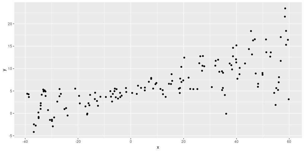
Figure 1: Simulated data
The task here is single-predictor regression, which in principle we can achieve use Keras dense layers.
Let’s see how to enhance this by indicating uncertainty, starting from the aleatoric type.
Aleatoric uncertainty
Aleatoric uncertainty, by definition, is not a statement about the model. So why not have the model learn the uncertainty inherent in the data?
This is exactly how aleatoric uncertainty is operationalized in this approach. Instead of a single output per input – the predicted mean of the regression – here we have two outputs: one for the mean, and one for the standard deviation.
How will we use these? Until shortly, we would have had to roll our own logic. Now with tfprobability, we make the network output not tensors, but distributions – put differently, we make the last layer a distribution layer.
Distribution layers are Keras layers, but contributed by tfprobability. The awesome thing is that we can train them with just tensors as targets, as usual: No need to compute probabilities ourselves.
Several specialized distribution layers exist, such as layer_kl_divergence_add_loss, layer_independent_bernoulli, or layer_mixture_same_family, but the most general is layer_distribution_lambda. layer_distribution_lambda takes as inputs the preceding layer and outputs a distribution. In order to be able to do this, we need to tell it how to make use of the preceding layer’s activations.
In our case, at some point we will want to have a dense layer with two units.
... %>% layer_dense(units = 2, activation = "linear") %>%Then layer_distribution_lambda will use the first unit as the mean of a normal distribution, and the second as its standard deviation.
layer_distribution_lambda(function(x)
    tfd_normal(loc = x[, 1, drop = FALSE],
               scale = 1e-3 + tf$math$softplus(x[, 2, drop = FALSE])
               )
)
Here is the complete model we use. We insert an additional dense layer in front, with a relu activation, to give the model a bit more freedom and capacity. We discuss this, as well as that scale = ... foo, as soon as we’ve finished our walkthrough of model training.
model <- keras_model_sequential() %>%
  layer_dense(units = 8, activation = "relu") %>%
  layer_dense(units = 2, activation = "linear") %>%
  layer_distribution_lambda(function(x)
    tfd_normal(loc = x[, 1, drop = FALSE],
               # ignore on first read, we'll come back to this
               # scale = 1e-3 + 0.05 * tf$math$softplus(x[, 2, drop = FALSE])
               scale = 1e-3 + tf$math$softplus(x[, 2, drop = FALSE])
               )
  )
For a model that outputs a distribution, the loss is the negative log likelihood given the target data.
negloglik <- function(y, model) - (model %>% tfd_log_prob(y))We can now compile and fit the model.
We now call the model on the test data to obtain the predictions. The predictions now actually are distributions, and we have 150 of them, one for each datapoint:
yhat <- model(tf$constant(x_test))tfp.distributions.Normal("sequential/distribution_lambda/Normal/",
batch_shape=[150, 1], event_shape=[], dtype=float32)To obtain the means and standard deviations – the latter being that measure of aleatoric uncertainty we’re interested in – we just call tfd_mean and tfd_stddev on these distributions. That will give us the predicted mean, as well as the predicted variance, per datapoint.
Let’s visualize this. Here are the actual test data points, the predicted means, as well as confidence bands indicating the mean estimate plus/minus two standard deviations.
ggplot(data.frame(
x = x,
y = y,
mean = as.numeric(mean),
sd = as.numeric(sd)
),
aes(x, y)) +
geom_point() +
geom_line(aes(x = x_test, y = mean), color = "violet", size = 1.5) +
geom_ribbon(aes(
x = x_test,
ymin = mean - 2 * sd,
ymax = mean + 2 * sd
),
alpha = 0.2,
fill = "grey")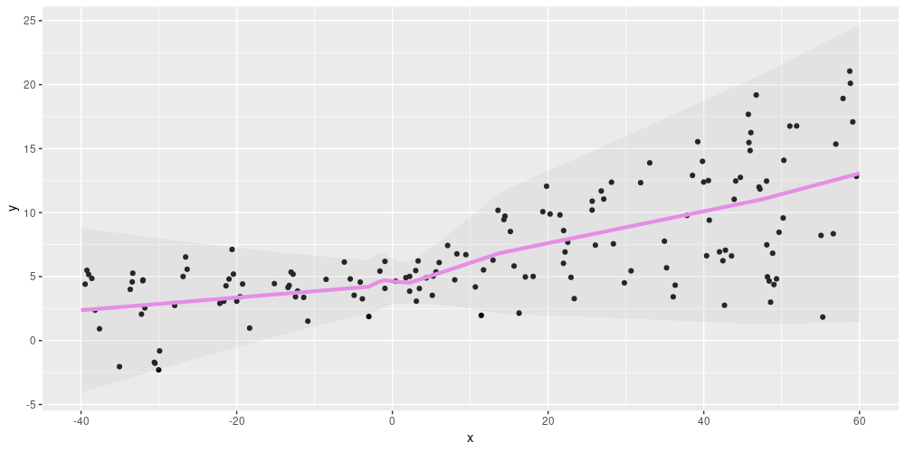
Figure 2: Aleatoric uncertainty on simulated data, using relu activation in the first dense layer.
This looks pretty reasonable. What if we had used linear activation in the first layer? Meaning, what if the model had looked like this2:
This time, the model does not capture the “form” of the data that well, as we’ve disallowed any nonlinearities.
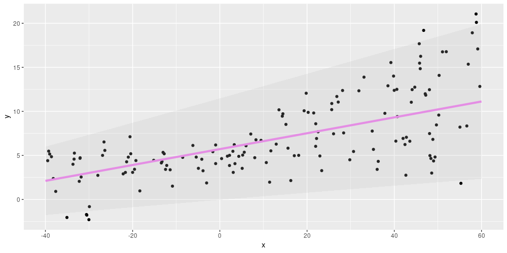
Figure 3: Aleatoric uncertainty on simulated data, using linear activation in the first dense layer.
Using linear activations only, we also need to do more experimenting with the scale = ... line to get the result look “right”. With relu, on the other hand, results are pretty robust to changes in how scale is computed. Which activation do we choose? If our goal is to adequately model variation in the data, we can just choose relu – and leave assessing uncertainty in the model to a different technique (the epistemic uncertainty that is up next).
Overall, it seems like aleatoric uncertainty is the straightforward part. We want the network to learn the variation inherent in the data, which it does. What do we gain? Instead of obtaining just point estimates, which in this example might turn out pretty bad in the two fan-like areas of the data on the left and right sides, we learn about the spread as well. We’ll thus be appropriately cautious depending on what input range we’re making predictions for.
Epistemic uncertainty
Now our focus is on the model. Given a speficic model (e.g., one from the linear family), what kind of data does it say conforms to its expectations?
To answer this question, we make use of a variational-dense layer.
This is again a Keras layer provided by tfprobability. Internally, it works by minimizing the evidence lower bound (ELBO), thus striving to find an approximative posterior that does two things:
- fit the actual data well (put differently: achieve high log likelihood), and
- stay close to a prior (as measured by KL divergence).
As users, we actually specify the form of the posterior as well as that of the prior. Here is how a prior could look.
prior_trainable <-
function(kernel_size,
bias_size = 0,
dtype = NULL) {
n <- kernel_size + bias_size
keras_model_sequential() %>%
# we'll comment on this soon
# layer_variable(n, dtype = dtype, trainable = FALSE) %>%
layer_variable(n, dtype = dtype, trainable = TRUE) %>%
layer_distribution_lambda(function(t) {
tfd_independent(tfd_normal(loc = t, scale = 1),
reinterpreted_batch_ndims = 1)
})
}This prior is itself a Keras model, containing a layer that wraps a variable and a layer_distribution_lambda, that type of distribution-yielding layer we’ve just encountered above. The variable layer could be fixed (non-trainable) or non-trainable, corresponding to a genuine prior or a prior learnt from the data in an empirical Bayes-like way. The distribution layer outputs a normal distribution since we’re in a regression setting.
The posterior too is a Keras model – definitely trainable this time. It too outputs a normal distribution:
posterior_mean_field <-
function(kernel_size,
bias_size = 0,
dtype = NULL) {
n <- kernel_size + bias_size
c <- log(expm1(1))
keras_model_sequential(list(
layer_variable(shape = 2 * n, dtype = dtype),
layer_distribution_lambda(
make_distribution_fn = function(t) {
tfd_independent(tfd_normal(
loc = t[1:n],
scale = 1e-5 + tf$nn$softplus(c + t[(n + 1):(2 * n)])
), reinterpreted_batch_ndims = 1)
}
)
))
}Now that we’ve defined both, we can set up the model’s layers. The first one, a variational-dense layer, has a single unit. The ensuing distribution layer then takes that unit’s output and uses it for the mean of a normal distribution – while the scale of that Normal is fixed at 1:
You may have noticed one argument to layer_dense_variational we haven’t discussed yet, kl_weight.
This is used to scale the contribution to the total loss of the KL divergence, and normally should equal one over the number of data points.
Training the model is straightforward. As users, we only specify the negative log likelihood part of the loss; the KL divergence part is taken care of transparently by the framework.
Because of the stochasticity inherent in a variational-dense layer, each time we call this model, we obtain different results: different normal distributions, in this case. To obtain the uncertainty estimates we’re looking for, we therefore call the model a bunch of times – 100, say:
yhats <- purrr::map(1:100, function(x) model(tf$constant(x_test)))We can now plot those 100 predictions – lines, in this case, as there are no nonlinearities:
means <-
purrr::map(yhats, purrr::compose(as.matrix, tfd_mean)) %>% abind::abind()
lines <- data.frame(cbind(x_test, means)) %>%
gather(key = run, value = value,-X1)
mean <- apply(means, 1, mean)
ggplot(data.frame(x = x, y = y, mean = as.numeric(mean)), aes(x, y)) +
geom_point() +
geom_line(aes(x = x_test, y = mean), color = "violet", size = 1.5) +
geom_line(
data = lines,
aes(x = X1, y = value, color = run),
alpha = 0.3,
size = 0.5
) +
theme(legend.position = "none")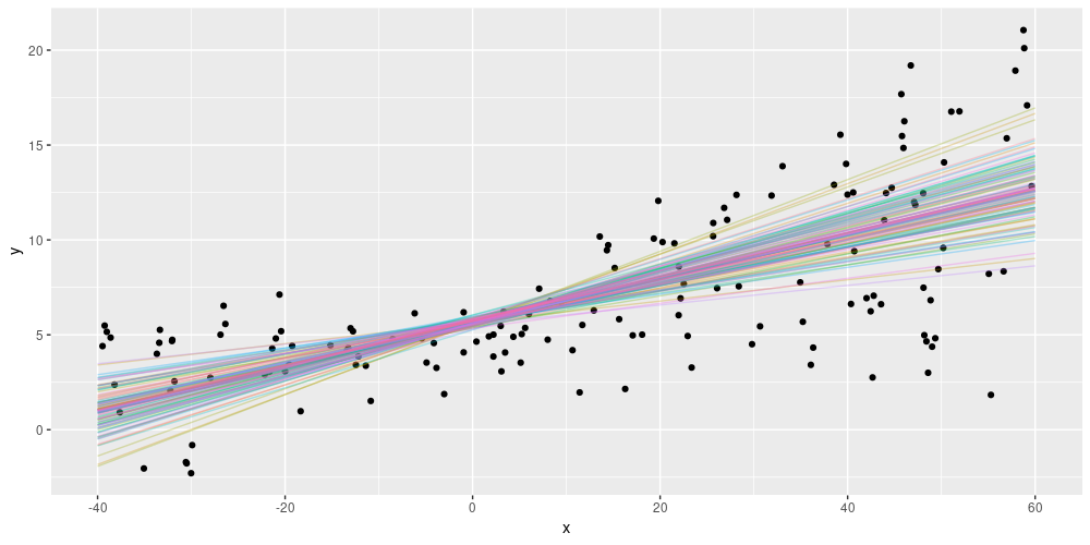
Figure 4: Epistemic uncertainty on simulated data, using linear activation in the variational-dense layer.
What we see here are essentially different models, consistent with the assumptions built into the architecture. What we’re not accounting for is the spread in the data. Can we do both? We can; but first let’s comment on a few choices that were made and see how they affect the results.
To prevent this post from growing to infinite size, we’ve refrained from performing a systematic experiment; please take what follows not as generalizable statements, but as pointers to things you will want to keep in mind in your own ventures. Especially, each (hyper-)parameter is not an island; they could interact in unforeseen ways.
After those words of caution, here are some things we noticed.
- One question you might ask: Before, in the aleatoric uncertainty setup, we added an additional dense layer to the model, with
reluactivation. What if we did this here? Firstly, we’re not adding any additional, non-variational layers in order to keep the setup “fully Bayesian” – we want priors at every level. As to usingreluinlayer_dense_variational, we did try that, and the results look pretty similar:
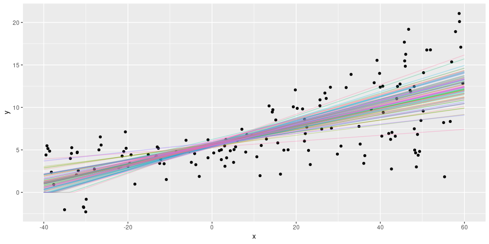
Figure 5: Epistemic uncertainty on simulated data, using relu activation in the variational-dense layer.
However, things look pretty different if we drastically reduce training time… which brings us to the next observation.
- Unlike in the aleatoric setup, the number of training epochs matter a lot. If we train, quote unquote, too long, the posterior estimates will get closer and closer to the posterior mean: we lose uncertainty. What happens if we train “too short” is even more notable. Here are the results for the linear-activation as well as the relu-activation cases:
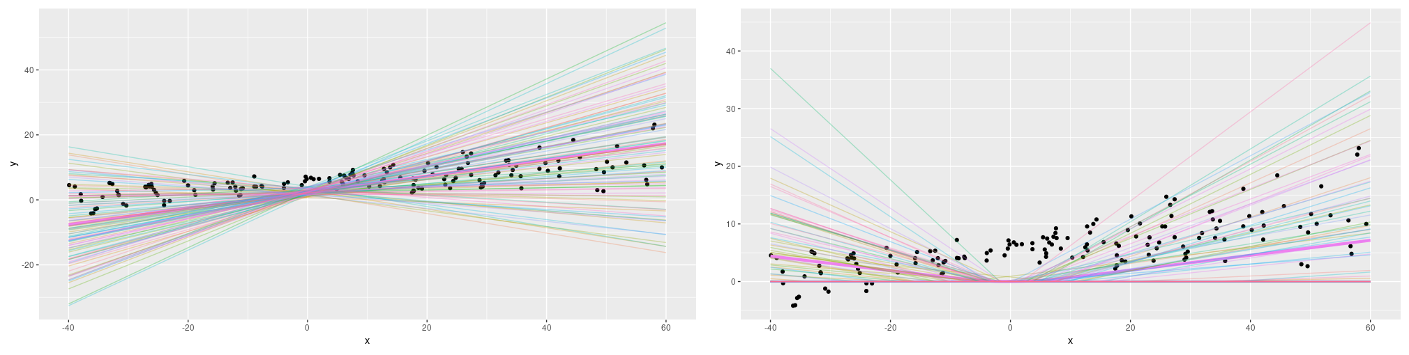
Figure 6: Epistemic uncertainty on simulated data if we train for 100 epochs only. Left: linear activation. Right: relu activation.
Interestingly, both model families look very different now, and while the linear-activation family looks more reasonable at first, it still considers an overall negative slope consistent with the data.
So how many epochs are “long enough”? From observation, we’d say that a working heuristic should probably be based on the rate of loss reduction. But certainly, it’ll make sense to try different numbers of epochs and check the effect on model behavior. As an aside, monitoring estimates over training time may even yield important insights into the assumptions built into a model (e.g., the effect of different activation functions).
As important as the number of epochs trained, and similar in effect, is the learning rate. If we replace the learning rate in this setup by
0.001, results will look similar to what we saw above for theepochs = 100case. Again, we will want to try different learning rates and make sure we train the model “to completion” in some reasonable sense.To conclude this section, let’s quickly look at what happens if we vary two other parameters. What if the prior were non-trainable (see the commented line above)? And what if we scaled the importance of the KL divergence (
kl_weightinlayer_dense_variational’s argument list) differently, replacingkl_weight = 1/nbykl_weight = 1(or equivalently, removing it)? Here are the respective results for an otherwise-default setup. They don’t lend themselves to generalization – on different (e.g., bigger!) datasets the outcomes will most certainly look different – but definitely interesting to observe.
Figure 7: Epistemic uncertainty on simulated data. Left: kl_weight = 1. Right: prior non-trainable.
Now let’s come back to the question: We’ve modeled spread in the data, we’ve peeked into the heart of the model, – can we do both at the same time?
We can, if we combine both approaches. We add an additional unit to the variational-dense layer and use this to learn the variance: once for each “sub-model” contained in the model.
Combining both aleatoric and epistemic uncertainty
Reusing the prior and posterior from above, this is how the final model looks:
model <- keras_model_sequential() %>%
layer_dense_variational(
units = 2,
make_posterior_fn = posterior_mean_field,
make_prior_fn = prior_trainable,
kl_weight = 1 / n
) %>%
layer_distribution_lambda(function(x)
tfd_normal(loc = x[, 1, drop = FALSE],
scale = 1e-3 + tf$math$softplus(0.01 * x[, 2, drop = FALSE])
)
)We train this model just like the epistemic-uncertainty only one. We then obtain a measure of uncertainty per predicted line. Or in the words we used above, we now have an ensemble of models each with its own indication of spread in the data. Here is a way we could display this – each colored line is the mean of a distribution, surrounded by a confidence band indicating +/- two standard deviations.
yhats <- purrr::map(1:100, function(x) model(tf$constant(x_test)))
means <-
purrr::map(yhats, purrr::compose(as.matrix, tfd_mean)) %>% abind::abind()
sds <-
purrr::map(yhats, purrr::compose(as.matrix, tfd_stddev)) %>% abind::abind()
means_gathered <- data.frame(cbind(x_test, means)) %>%
gather(key = run, value = mean_val,-X1)
sds_gathered <- data.frame(cbind(x_test, sds)) %>%
gather(key = run, value = sd_val,-X1)
lines <-
means_gathered %>% inner_join(sds_gathered, by = c("X1", "run"))
mean <- apply(means, 1, mean)
ggplot(data.frame(x = x, y = y, mean = as.numeric(mean)), aes(x, y)) +
geom_point() +
theme(legend.position = "none") +
geom_line(aes(x = x_test, y = mean), color = "violet", size = 1.5) +
geom_line(
data = lines,
aes(x = X1, y = mean_val, color = run),
alpha = 0.6,
size = 0.5
) +
geom_ribbon(
data = lines,
aes(
x = X1,
ymin = mean_val - 2 * sd_val,
ymax = mean_val + 2 * sd_val,
group = run
),
alpha = 0.05,
fill = "grey",
inherit.aes = FALSE
)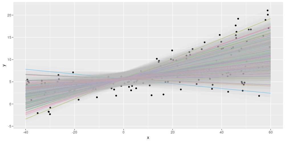
Figure 8: Displaying both epistemic and aleatoric uncertainty on the simulated dataset.
Nice! This looks like something we could report.
As you might imagine, this model, too, is sensitive to how long (think: number of epochs) or how fast (think: learning rate) we train it. And compared to the epistemic-uncertainty only model, there is an additional choice to be made here: the scaling of the previous layer’s activation – the 0.01 in the scale argument to tfd_normal:
scale = 1e-3 + tf$math$softplus(0.01 * x[, 2, drop = FALSE])Keeping everything else constant, here we vary that parameter between 0.01 and 0.05:
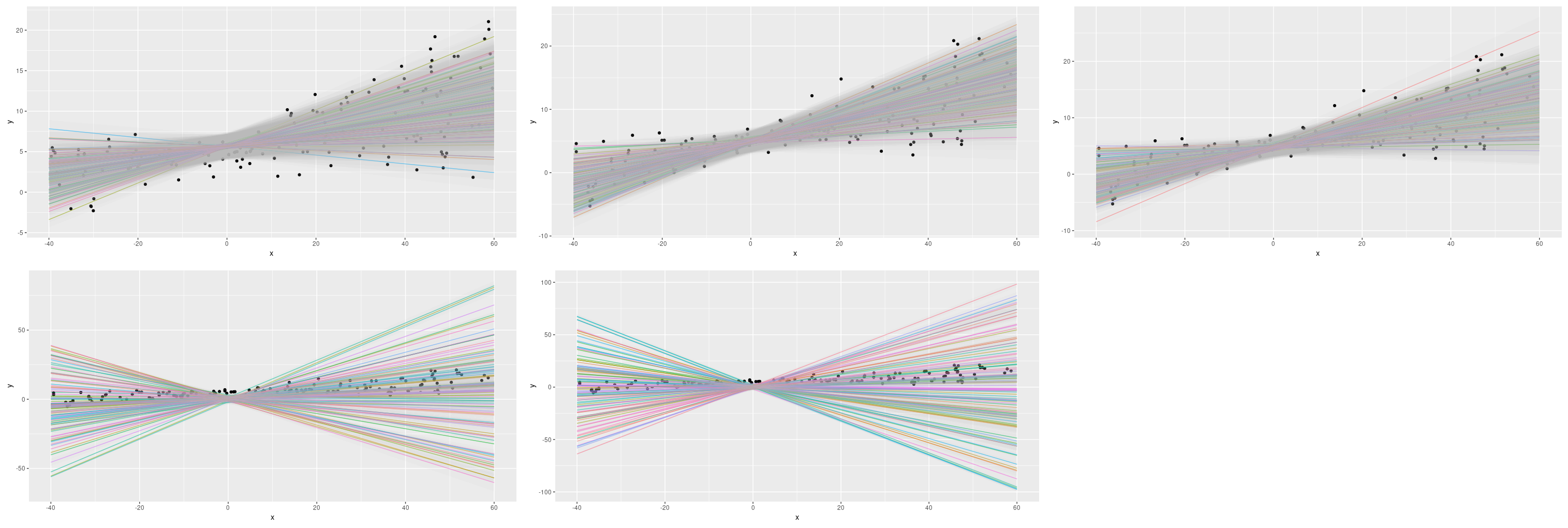
Figure 9: Epistemic plus aleatoric uncertainty on the simulated dataset: Varying the scale argument.
Evidently, this is another parameter we should be prepared to experiment with.
Now that we’ve introduced all three types of presenting uncertainty – aleatoric only, epistemic only, or both – let’s see them on the aforementioned Combined Cycle Power Plant Data Set. Please see our previous post on uncertainty for a quick characterization, as well as visualization, of the dataset.
Combined Cycle Power Plant Data Set
To keep this post at a digestible length, we’ll refrain from trying as many alternatives as with the simulated data and mainly stay with what worked well there. This should also give us an idea of how well these “defaults” generalize. We separately inspect two scenarios: The single-predictor setup (using each of the four available predictors alone), and the complete one (using all four predictors at once).
The dataset is loaded just as in the previous post.
library(tensorflow)
library(tfprobability)
library(keras)
library(dplyr)
library(tidyr)
library(readxl)
# make sure this code is compatible with TensorFlow 2.0
tf$compat$v1$enable_v2_behavior()
df <- read_xlsx("CCPP/Folds5x2_pp.xlsx")
df_scaled <- scale(df)
centers <- attr(df_scaled, "scaled:center")
scales <- attr(df_scaled, "scaled:scale")
X <- df_scaled[, 1:4]
train_samples <- sample(1:nrow(df_scaled), 0.8 * nrow(X))
X_train <- X[train_samples, ]
X_val <- X[-train_samples, ]
y <- df_scaled[, 5]
y_train <- y[train_samples] %>% as.matrix()
y_val <- y[-train_samples] %>% as.matrix()First we look at the single-predictor case, starting from aleatoric uncertainty.
Single predictor: Aleatoric uncertainty
Here is the “default” aleatoric model again. We also duplicate the plotting code here for the reader’s convenience.
n <- nrow(X_train) # 7654
n_epochs <- 10 # we need fewer epochs because the dataset is so much bigger
batch_size <- 100
learning_rate <- 0.01
# variable to fit - change to 2,3,4 to get the other predictors
i <- 1
model <- keras_model_sequential() %>%
layer_dense(units = 16, activation = "relu") %>%
layer_dense(units = 2, activation = "linear") %>%
layer_distribution_lambda(function(x)
tfd_normal(loc = x[, 1, drop = FALSE],
scale = tf$math$softplus(x[, 2, drop = FALSE])
)
)
negloglik <- function(y, model) - (model %>% tfd_log_prob(y))
model %>% compile(optimizer = optimizer_adam(lr = learning_rate), loss = negloglik)
hist <-
model %>% fit(
X_train[, i, drop = FALSE],
y_train,
validation_data = list(X_val[, i, drop = FALSE], y_val),
epochs = n_epochs,
batch_size = batch_size
)
yhat <- model(tf$constant(X_val[, i, drop = FALSE]))
mean <- yhat %>% tfd_mean()
sd <- yhat %>% tfd_stddev()
ggplot(data.frame(
x = X_val[, i],
y = y_val,
mean = as.numeric(mean),
sd = as.numeric(sd)
),
aes(x, y)) +
geom_point() +
geom_line(aes(x = x, y = mean), color = "violet", size = 1.5) +
geom_ribbon(aes(
x = x,
ymin = mean - 2 * sd,
ymax = mean + 2 * sd
),
alpha = 0.4,
fill = "grey")How well does this work?
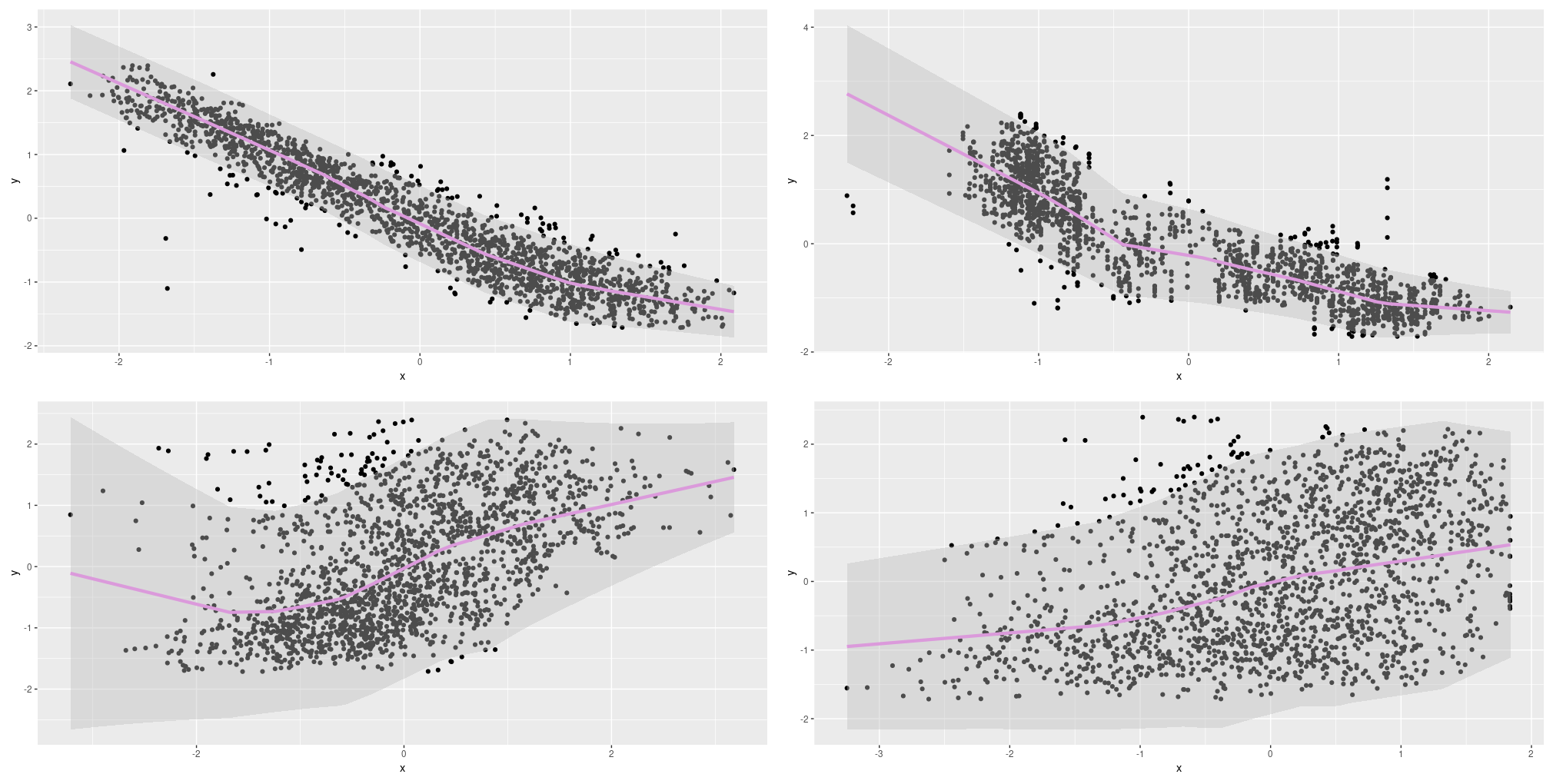
Figure 10: Aleatoric uncertainty on the Combined Cycle Power Plant Data Set; single predictors.
This looks pretty good we’d say! How about epistemic uncertainty?
Single predictor: Epistemic uncertainty
Here’s the code:
posterior_mean_field <-
  function(kernel_size,
           bias_size = 0,
           dtype = NULL) {
    n <- kernel_size + bias_size
    c <- log(expm1(1))
    keras_model_sequential(list(
      layer_variable(shape = 2 * n, dtype = dtype),
      layer_distribution_lambda(
        make_distribution_fn = function(t) {
          tfd_independent(tfd_normal(
            loc = t[1:n],
            scale = 1e-5 + tf$nn$softplus(c + t[(n + 1):(2 * n)])
            ), reinterpreted_batch_ndims = 1)
        }
      )
    ))
  }
prior_trainable <-
function(kernel_size,
bias_size = 0,
dtype = NULL) {
n <- kernel_size + bias_size
keras_model_sequential() %>%
layer_variable(n, dtype = dtype, trainable = TRUE) %>%
layer_distribution_lambda(function(t) {
tfd_independent(tfd_normal(loc = t, scale = 1),
reinterpreted_batch_ndims = 1)
})
}
model <- keras_model_sequential() %>%
layer_dense_variational(
units = 1,
make_posterior_fn = posterior_mean_field,
make_prior_fn = prior_trainable,
kl_weight = 1 / n,
activation = "linear",
) %>%
layer_distribution_lambda(function(x)
tfd_normal(loc = x, scale = 1))
negloglik <- function(y, model) - (model %>% tfd_log_prob(y))
model %>% compile(optimizer = optimizer_adam(lr = learning_rate), loss = negloglik)
hist <-
model %>% fit(
X_train[, i, drop = FALSE],
y_train,
validation_data = list(X_val[, i, drop = FALSE], y_val),
epochs = n_epochs,
batch_size = batch_size
)
yhats <- purrr::map(1:100, function(x)
yhat <- model(tf$constant(X_val[, i, drop = FALSE])))
means <-
purrr::map(yhats, purrr::compose(as.matrix, tfd_mean)) %>% abind::abind()
lines <- data.frame(cbind(X_val[, i], means)) %>%
gather(key = run, value = value,-X1)
mean <- apply(means, 1, mean)
ggplot(data.frame(x = X_val[, i], y = y_val, mean = as.numeric(mean)), aes(x, y)) +
geom_point() +
geom_line(aes(x = X_val[, i], y = mean), color = "violet", size = 1.5) +
geom_line(
data = lines,
aes(x = X1, y = value, color = run),
alpha = 0.3,
size = 0.5
) +
theme(legend.position = "none")And this is the result.
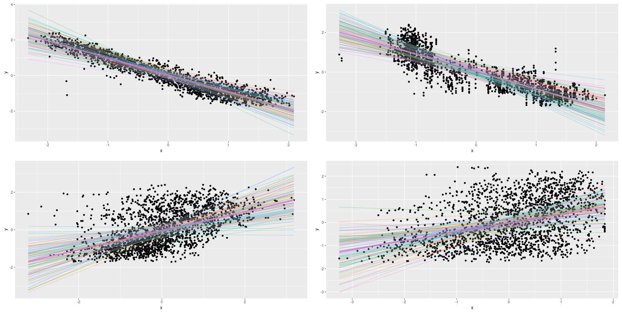
Figure 11: Epistemic uncertainty on the Combined Cycle Power Plant Data Set; single predictors.
As with the simulated data, the linear models seems to “do the right thing”. And here too, we think we will want to augment this with the spread in the data: Thus, on to way three.
Single predictor: Combining both types
Here we go. Again, posterior_mean_field and prior_trainable look just like in the epistemic-only case.
model <- keras_model_sequential() %>%
  layer_dense_variational(
    units = 2,
    make_posterior_fn = posterior_mean_field,
    make_prior_fn = prior_trainable,
    kl_weight = 1 / n,
    activation = "linear"
  ) %>%
  layer_distribution_lambda(function(x)
    tfd_normal(loc = x[, 1, drop = FALSE],
               scale = 1e-3 + tf$math$softplus(0.01 * x[, 2, drop = FALSE])))


negloglik <- function(y, model)
  - (model %>% tfd_log_prob(y))
model %>% compile(optimizer = optimizer_adam(lr = learning_rate), loss = negloglik)
hist <-
  model %>% fit(
    X_train[, i, drop = FALSE],
    y_train,
    validation_data = list(X_val[, i, drop = FALSE], y_val),
    epochs = n_epochs,
    batch_size = batch_size
  )

yhats <- purrr::map(1:100, function(x)
  model(tf$constant(X_val[, i, drop = FALSE])))
means <-
  purrr::map(yhats, purrr::compose(as.matrix, tfd_mean)) %>% abind::abind()
sds <-
  purrr::map(yhats, purrr::compose(as.matrix, tfd_stddev)) %>% abind::abind()

means_gathered <- data.frame(cbind(X_val[, i], means)) %>%
  gather(key = run, value = mean_val,-X1)
sds_gathered <- data.frame(cbind(X_val[, i], sds)) %>%
  gather(key = run, value = sd_val,-X1)

lines <-
  means_gathered %>% inner_join(sds_gathered, by = c("X1", "run"))

mean <- apply(means, 1, mean)

#lines <- lines %>% filter(run=="X3" | run =="X4")

ggplot(data.frame(x = X_val[, i], y = y_val, mean = as.numeric(mean)), aes(x, y)) +
  geom_point() +
  theme(legend.position = "none") +
  geom_line(aes(x = X_val[, i], y = mean), color = "violet", size = 1.5) +
  geom_line(
    data = lines,
    aes(x = X1, y = mean_val, color = run),
    alpha = 0.2,
    size = 0.5
  ) +
geom_ribbon(
  data = lines,
  aes(
    x = X1,
    ymin = mean_val - 2 * sd_val,
    ymax = mean_val + 2 * sd_val,
    group = run
  ),
  alpha = 0.01,
  fill = "grey",
  inherit.aes = FALSE
)
And the output?
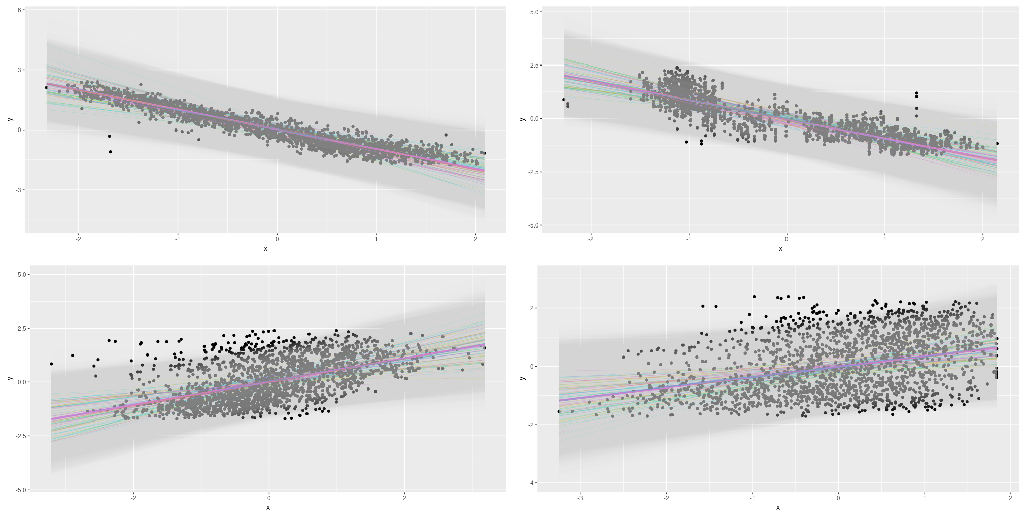
Figure 12: Combined uncertainty on the Combined Cycle Power Plant Data Set; single predictors.
This looks useful! Let’s wrap up with our final test case: Using all four predictors together.
All predictors
The training code used in this scenario looks just like before, apart from our feeding all predictors to the model. For plotting, we resort to displaying the first principal component on the x-axis – this makes the plots look noisier than before. We also display fewer lines for the epistemic and epistemic-plus-aleatoric cases (20 instead of 100). Here are the results:
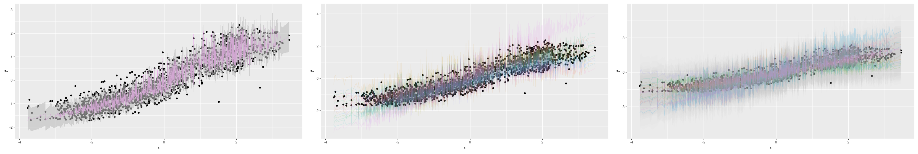
Figure 13: Uncertainty (aleatoric, epistemic, both) on the Combined Cycle Power Plant Data Set; all predictors.
Conclusion
Where does this leave us? Compared to the learnable-dropout approach described in the prior post, the way presented here is a lot easier, faster, and more intuitively understandable. The methods per se are that easy to use that in this first introductory post, we could afford to explore alternatives already: something we had no time to do in that previous exposition.
In fact, we hope this post leaves you in a position to do your own experiments, on your own data. Obviously, you will have to make decisions, but isn’t that the way it is in data science? There’s no way around making decisions; we just should be prepared to justify them … Thanks for reading!