What could be treacherous about summary statistics?
The famous cat overweight study (X. et al., 2019) showed that as of May 1st, 2019, 32 of 101 domestic cats held in Y., a cozy Bavarian village, were overweight. Even though I’d be curious to know if my aunt G.’s cat (a happy resident of that village) has been fed too many treats and has accumulated some excess pounds, the study results don’t tell.
Then, six months later, out comes a new study, ambitious to earn scientific fame. The authors report that of 100 cats living in Y., 50 are striped, 31 are black, and the rest are white; the 31 black ones are all overweight. Now, I happen to know that, with one exception, no new cats joined the community, and no cats left. But, my aunt moved away to a retirement home, chosen of course for the possibility to bring one’s cat.
What have I just learned? My aunt’s cat is overweight. (Or was, at least, before they moved to the retirement home.)
Even though none of the studies reported anything but summary statistics, I was able to infer individual-level facts by connecting both studies and adding in another piece of information I had access to.
In reality, mechanisms like the above – technically called linkage – have been shown to lead to privacy breaches many times, thus defeating the purpose of database anonymization seen as a panacea in many organizations. A more promising alternative is offered by the concept of differential privacy.
Differential Privacy
In differential privacy (DP)1(Dwork et al. 2006), privacy is not a property of what’s in the database; it’s a property of how query results are delivered.
Intuitively paraphrasing results from a domain where results are communicated as theorems and proofs (Dwork 2006)(Dwork and Roth 2014), the only achievable (in a lossy but quantifiable way) objective is that from queries to a database, nothing more should be learned about an individual in that database than if they hadn’t been in there at all.(Wood et al. 2018)
What this statement does is caution against overly high expectations: Even if query results are reported in a DP way (we’ll see how that goes in a second), they enable some probabilistic inferences about individuals in the respective population. (Otherwise, why conduct studies at all.)
So how is DP being achieved? The main ingredient is noise added to the results of a query. In the above cat example, instead of exact numbers we’d report approximate ones: “Of ~ 100 cats living in Y, about 30 are overweight….” If this is done for both of the above studies, no inference will be possible about aunt G.’s cat.
Even with random noise added to query results though, answers to repeated queries will leak information. So in reality, there is a privacy budget that can be tracked, and may be used up in the course of consecutive queries.
This is reflected in the formal definition of DP. The idea is that queries to two databases differing in at most one element should give basically the same result. Put formally (Dwork 2006):
A randomized function \(\mathcal{K}\) gives \(\epsilon\) -differential privacy if for all data sets D1 and D2 differing on at most one element, and all \(S \subseteq Range(K)\),
\(Pr[\mathcal{K}(D1)\in S] \leq exp(\epsilon) × Pr[K(D2) \in S]\)
This \(\epsilon\) -differential privacy is additive: If one query is \(\epsilon\)-DP at a value of 0.01, and another one at 0.03, together they will be 0.04 \(\epsilon\)-differentially private.
If \(\epsilon\)-DP is to be achieved via adding noise, how exactly should this be done? Here, several mechanisms exist; the basic, intuitively plausible principle though is that the amount of noise should be calibrated to the target function’s sensitivity, defined as the maximum \(\ell 1\) norm of the difference of function values computed on all pairs of datasets differing in a single example (Dwork 2006):
\(\Delta f = \max_{D1,D2} {\| f(D1)−f(D2) \|}_1\)
So far, we’ve been talking about databases and datasets. How does this apply to machine and/or deep learning?
TensorFlow Privacy
Applying DP to deep learning, we want a model’s parameters to wind up “essentially the same” whether trained on a dataset including that cute little kitty or not. TensorFlow (TF) Privacy (Abadi et al. 2016), a library built on top of TF, makes it easy on users to add privacy guarantees to their models – easy, that is, from a technical point of view. (As with life overall, the hard decisions on how much of an asset we should be reaching for, and how to trade off one asset (here: privacy) with another (here: model performance), remain to be taken by each of us ourselves.)
Concretely, about all we have to do is exchange the optimizer we were using against one provided by TF Privacy.2 TF Privacy optimizers wrap the original TF ones, adding two actions:
To honor the principle that each individual training example should have just moderate influence on optimization, gradients are clipped (to a degree specifiable by the user). In contrast to the familiar gradient clipping sometimes used to prevent exploding gradients, what is clipped here is gradient contribution per user.
Before updating the parameters, noise is added to the gradients, thus implementing the main idea of \(\epsilon\)-DP algorithms.
In addition to \(\epsilon\)-DP optimization, TF Privacy provides privacy accounting. We’ll see all this applied after an introduction to our example dataset.
Dataset
The dataset we’ll be working with(Reiss et al. 2019), downloadable from the UCI Machine Learning Repository, is dedicated to heart rate estimation via photoplethysmography. Photoplethysmography (PPG) is an optical method of measuring blood volume changes in the microvascular bed of tissue, which are indicative of cardiovascular activity. More precisely,
The PPG waveform comprises a pulsatile (‘AC’) physiological waveform attributed to cardiac synchronous changes in the blood volume with each heart beat, and is superimposed on a slowly varying (‘DC’) baseline with various lower frequency components attributed to respiration, sympathetic nervous system activity and thermoregulation. (Allen 2007)
In this dataset, heart rate determined from EKG provides the ground truth; predictors were obtained from two commercial devices, comprising PPG, electrodermal activity, body temperature as well as accelerometer data. Additionally, a wealth of contextual data is available, ranging from age, height, and weight to fitness level and type of activity performed.
With this data, it’s easy to imagine a bunch of interesting data-analysis questions; however here our focus is on differential privacy, so we’ll keep the setup simple. We will try to predict heart rate given the physiological measurements from one of the two devices, Empatica E4. Also, we’ll zoom in on a single subject, S1, who will provide us with 4603 instances of two-second heart rate values.3
As usual, we start with the required libraries; unusually though, as of this writing we need to disable version 2 behavior in TensorFlow, as TensorFlow Privacy does not yet fully work with TF 2. (Hopefully, for many future readers, this won’t be the case anymore.)
Note how TF Privacy – a Python library – is imported via reticulate.
library(tensorflow)
tf$compat$v1$disable_v2_behavior()

library(keras)
library(tfdatasets)
library(tfautograph)

library(purrr)

library(reticulate)
# if you haven't yet, install TF Privacy, e.g. using reticulate:
# py_install("tensorflow_privacy")
priv <- import("tensorflow_privacy")
From the downloaded archive, we just need S1.pkl, saved in a native Python serialization format, yet nicely loadable using reticulate:
s1 <- py_load_object("PPG_FieldStudy/S1/S1.pkl", encoding = "latin1")s1 points to an R list comprising elements of different length – the various physical/physiological signals have been sampled with different frequencies:
### predictors ###

# accelerometer data - sampling freq. 32 Hz
# also note that these are 3 "columns", for each of x, y, and z axes
s1$signal$wrist$ACC %>% nrow() # 294784
# PPG data - sampling freq. 64 Hz
s1$signal$wrist$BVP %>% nrow() # 589568
# electrodermal activity data - sampling freq. 4 Hz
s1$signal$wrist$EDA %>% nrow() # 36848
# body temperature data - sampling freq. 4 Hz
s1$signal$wrist$TEMP %>% nrow() # 36848

### target ###

# EKG data - provided in already averaged form, at frequency 0.5 Hz
s1$label %>% nrow() # 4603
In light of the different sampling frequencies, our tfdatasets pipeline will have do some moving averaging, paralleling that applied to construct the ground truth data.
Preprocessing pipeline
As every “column”4 is of different length and resolution, we build up the final dataset piece-by-piece. The following function serves two purposes:
- compute running averages over differently sized windows, thus downsampling to 0.5Hz for every modality
- transform the data to the
(num_timesteps, num_features)format that will be required by the 1d-convnet we’re going to use soon
average_and_make_sequences <-
  function(data, window_size_avg, num_timesteps) {
    data %>% k_cast("float32") %>%
      # create an initial tf.data dataset to work with
      tensor_slices_dataset() %>%
      # use dataset_window to compute the running average of size window_size_avg
      dataset_window(window_size_avg) %>%
      dataset_flat_map(function (x)
        x$batch(as.integer(window_size_avg), drop_remainder = TRUE)) %>%
      dataset_map(function(x)
        tf$reduce_mean(x, axis = 0L)) %>%
      # use dataset_window to create a "timesteps" dimension with length num_timesteps)
      dataset_window(num_timesteps, shift = 1) %>%
      dataset_flat_map(function(x)
        x$batch(as.integer(num_timesteps), drop_remainder = TRUE))
  }
We’ll call this function for every column separately. Not all columns are exactly the same length (in terms of time), thus it’s safest to cut off individual observations that surpass a common length (dictated by the target variable):
label <- s1$label %>% matrix() # 4603 observations, each spanning 2 secs
n_total <- 4603 # keep track of this

# keep matching numbers of observations of predictors
acc <- s1$signal$wrist$ACC[1:(n_total * 64), ] # 32 Hz, 3 columns
bvp <- s1$signal$wrist$BVP[1:(n_total * 128)] %>% matrix() # 64 Hz
eda <- s1$signal$wrist$EDA[1:(n_total * 8)] %>% matrix() # 4 Hz
temp <- s1$signal$wrist$TEMP[1:(n_total * 8)] %>% matrix() # 4 Hz
Some more housekeeping. Both training and the test set need to have a timesteps dimension, as usual with architectures that work on sequential data (1-d convnets and RNNs). To make sure there is no overlap between respective timesteps, we split the data “up front” and assemble both sets separately. We’ll use the first 4000 observations for training.
Housekeeping-wise, we also keep track of actual training and test set cardinalities. The target variable will be matched to the last of any twelve timesteps, so we end up throwing away the first eleven ground truth measurements for each of the training and test datasets. (We don’t have complete sequences building up to them.)
# number of timesteps used in the second dimension
num_timesteps <- 12

# number of observations to be used for the training set
# a round number for easier checking!
train_max <- 4000

# also keep track of actual number of training and test observations
n_train <- train_max - num_timesteps + 1
n_test <- n_total - train_max - num_timesteps + 1
Here, then, are the basic building blocks that will go into the final training and test datasets.
acc_train <-
  average_and_make_sequences(acc[1:(train_max * 64), ], 64, num_timesteps)
bvp_train <-
  average_and_make_sequences(bvp[1:(train_max * 128), , drop = FALSE], 128, num_timesteps)
eda_train <-
  average_and_make_sequences(eda[1:(train_max * 8), , drop = FALSE], 8, num_timesteps)
temp_train <-
  average_and_make_sequences(temp[1:(train_max * 8), , drop = FALSE], 8, num_timesteps)


acc_test <-
  average_and_make_sequences(acc[(train_max * 64 + 1):nrow(acc), ], 64, num_timesteps)
bvp_test <-
  average_and_make_sequences(bvp[(train_max * 128 + 1):nrow(bvp), , drop = FALSE], 128, num_timesteps)
eda_test <-
  average_and_make_sequences(eda[(train_max * 8 + 1):nrow(eda), , drop = FALSE], 8, num_timesteps)
temp_test <-
  average_and_make_sequences(temp[(train_max * 8 + 1):nrow(temp), , drop = FALSE], 8, num_timesteps)
Now put all predictors together:
On the ground truth side, as alluded to before, we leave out the first eleven values in each case:
y_train <- tensor_slices_dataset(label[num_timesteps:train_max] %>% k_cast("float32"))

y_test <- tensor_slices_dataset(label[(train_max + num_timesteps):nrow(label)] %>% k_cast("float32")
Zip predictors and targets together, configure shuffling/batching, and the datasets are complete:
ds_train <- zip_datasets(x_train, y_train)
ds_test <- zip_datasets(x_test, y_test)

batch_size <- 32

ds_train <- ds_train %>%
  dataset_shuffle(n_train) %>%
  # dataset_repeat is needed because of pre-TF 2 style
  # hopefully at a later time, the code can run eagerly and this is no longer needed
  dataset_repeat() %>%
  dataset_batch(batch_size, drop_remainder = TRUE)

ds_test <- ds_test %>%
  # see above reg. dataset_repeat
  dataset_repeat() %>%
  dataset_batch(batch_size)
With data manipulations as complicated as the above, it’s always worthwhile checking some pipeline outputs. We can do that using the usual reticulate::as_iterator magic, provided that for this test run, we don’t disable V2 behavior. (Just restart the R session between a “pipeline checking” and the later modeling runs.)
Here, in any case, would be the relevant code:
# this piece needs TF 2 behavior enabled
# run after restarting R and commenting the tf$compat$v1$disable_v2_behavior() line
# then to fit the DP model, undo comment, restart R and rerun
iter <- as_iterator(ds_test) # or any other dataset you want to check
while (TRUE) {
 item <- iter_next(iter)
 if (is.null(item)) break
 print(item)
}
With that we’re ready to create the model.
Model
The model will be a rather simple convnet. The main difference between standard and DP training lies in the optimization procedure; thus, it’s straightforward to first establish a non-DP baseline. Later, when switching to DP, we’ll be able to reuse almost everything.
Here, then, is the model definition valid for both cases:
model <- keras_model_sequential() %>%
  layer_conv_1d(
      filters = 32,
      kernel_size = 3,
      activation = "relu"
    ) %>%
  layer_batch_normalization() %>%
  layer_conv_1d(
      filters = 64,
      kernel_size = 5,
      activation = "relu"
    ) %>%
  layer_batch_normalization() %>%
  layer_conv_1d(
      filters = 128,
      kernel_size = 5,
      activation = "relu"
    ) %>%
  layer_batch_normalization() %>%
  layer_global_average_pooling_1d() %>%
  layer_dense(units = 128, activation = "relu") %>%
  layer_dense(units = 1)
We train the model with mean squared error loss.
Baseline results
After 20 epochs, mean absolute error is around 6 bpm:
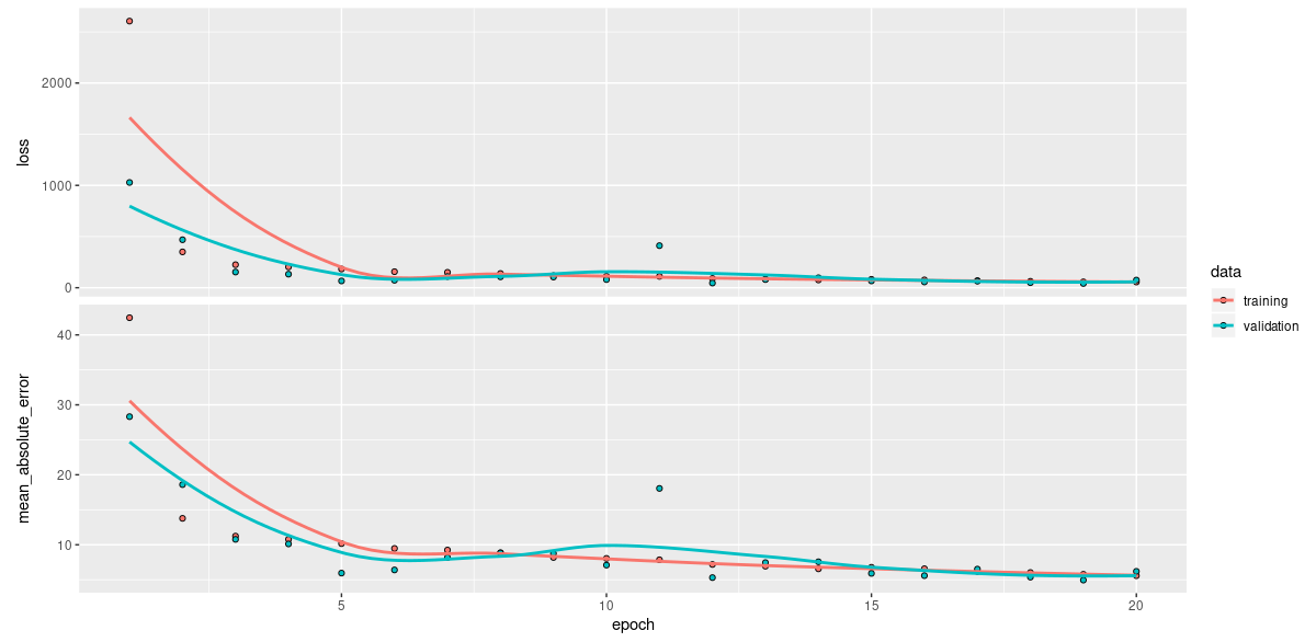
Figure 1: Training history without differential privacy.
Just to put this in context, the MAE reported for subject S1 in the paper(Reiss et al. 2019) – based on a higher-capacity network, extensive hyperparameter tuning, and naturally, training on the complete dataset – amounts to 8.45 bpm on average; so our setup seems to be sound.
Now we’ll make this differentially private.
DP training
Instead of the plain Adam optimizer, we use the corresponding TF Privacy wrapper, DPAdamGaussianOptimizer.
We need to tell it how aggressive gradient clipping should be (l2_norm_clip) and how much noise to add (noise_multiplier). Furthermore, we define the learning rate (there is no default), going for 10 times the default 0.001 based on initial experiments.
There is an additional parameter, num_microbatches, that could be used to speed up training (McMahan and Andrew 2018), but, as training duration is not an issue here, we just set it equal to batch_size.
The values for l2_norm_clip and noise_multiplier chosen here follow those used in the tutorials in the TF Privacy repo.
Nicely, TF Privacy comes with a script that allows one to compute the attained \(\epsilon\) beforehand, based on number of training examples, batch_size, noise_multiplier and number of training epochs.5
Calling that script, and assuming we train for 20 epochs here as well,
python compute_dp_sgd_privacy.py --N=3989 --batch_size=32 --noise_multiplier=1.1 --epochs=20this is what we get back:
DP-SGD with sampling rate = 0.802% and noise_multiplier = 1.1 iterated over
2494 steps satisfies differential privacy with eps = 2.73 and delta = 1e-06.
How good is a value of 2.73? Citing the TF Privacy authors:
\(\epsilon\) gives a ceiling on how much the probability of a particular output can increase by including (or removing) a single training example. We usually want it to be a small constant (less than 10, or, for more stringent privacy guarantees, less than 1). However, this is only an upper bound, and a large value of epsilon may still mean good practical privacy.
Obviously, choice of \(\epsilon\) is a (challenging) topic unto itself, and not something we can elaborate on in a post dedicated to the technical aspects of DP with TensorFlow.
How would \(\epsilon\) change if we trained for 50 epochs instead? (This is actually what we’ll do, seeing that training results on the test set tend to jump around quite a bit.)
python compute_dp_sgd_privacy.py --N=3989 --batch_size=32 --noise_multiplier=1.1 --epochs=60DP-SGD with sampling rate = 0.802% and noise_multiplier = 1.1 iterated over
6233 steps satisfies differential privacy with eps = 4.25 and delta = 1e-06.Having talked about its parameters, now let’s define the DP optimizer:
l2_norm_clip <- 1
noise_multiplier <- 1.1
num_microbatches <- k_cast(batch_size, "int32")
learning_rate <- 0.01

optimizer <- priv$DPAdamGaussianOptimizer(
  l2_norm_clip = l2_norm_clip,
  noise_multiplier = noise_multiplier,
  num_microbatches = num_microbatches,
  learning_rate = learning_rate
)
There is one other change to make for DP. As gradients are clipped on a per-sample basis, the optimizer needs to work with per-sample losses as well:
loss <- tf$keras$losses$MeanSquaredError(reduction = tf$keras$losses$Reduction$NONE)Everything else stays the same. Training history (like we said above, lasting for 50 epochs now) looks a lot more turbulent, with MAEs on the test set fluctuating between 8 and 20 over the last 10 training epochs:
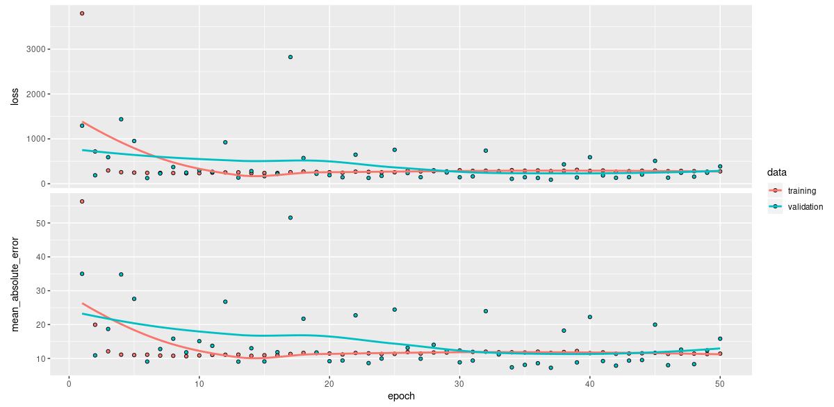
Figure 2: Training history with differential privacy.
In addition to the above-mentioned command line script, we can also compute \(\epsilon\) as part of the training code. Let’s double check:
# probability of an individual training point being included in a minibatch
sampling_probability <- batch_size / n_train

# number of steps the optimizer takes over the training data
steps <- num_epochs * n_train / batch_size

# required for reasons related to how TF Privacy computes privacy
# this actually is Renyi Differential Privacy: https://arxiv.org/abs/1702.07476
# we don't go into details here and use same values as the command line script
orders <- c((1 + (1:99)/10), 12:63)

rdp <- priv$privacy$analysis$rdp_accountant$compute_rdp(
  q = sampling_probability,
  noise_multiplier = noise_multiplier,
  steps = steps,
  orders = orders)

priv$privacy$analysis$rdp_accountant$get_privacy_spent(
  orders, rdp, target_delta = 1e-6)[[1]]
[1] 4.249645So, we do get the same result.
Conclusion
This post showed how to convert a normal deep learning procedure into an \(\epsilon\)-differentially private one. Necessarily, a blog post has to leave open questions. In the present case, some possible questions could be answered by straightforward experimentation:
- How well do other optimizers work in this setting?
- How does the learning rate affect privacy and performance?
- What happens if we train for a lot longer?
Others sound more like they could lead to a research project:
- When model performance – and thus, model parameters – fluctuate that much, how do we decide on when to stop training? Is stopping at high model performance cheating? Is model averaging a sound solution?
- How good really is any one \(\epsilon\)?
Finally, yet others transcend the realms of experimentation as well as mathematics:
- How do we trade off \(\epsilon\)-DP against model performance – for different applications, with different types of data, in different societal contexts?
- Assuming we “have” \(\epsilon\)-DP, what might we still be missing?
With questions like these – and more, probably – to ponder: Thanks for reading and a happy new year!
We’ll be using DP as an acronym for both the noun phrase “differential privacy” and the adjective phrase “differentially private.”↩︎
This is not exactly everything, as we’ll see when we get to the code, but “just about.”↩︎
Relative files per subject are 1.4G in size.↩︎
For convenience, we take the liberty to talk as if we had the usual rectangular data here.↩︎
There is an additional parameter, \(\delta\), that allows for bounding the risk that the privacy guarantee does not hold. The recommendation is to set this to at most the inverse of the number of training examples, which in out case would mean <= ~
1e-04; the default setting is1e-06so we should be fine here.↩︎