A Preamble, sort of
As we’re writing this – it’s April, 2023 – it is hard to overstate the attention going to, the hopes associated with, and the fears surrounding deep-learning-powered image and text generation. Impacts on society, politics, and human well-being deserve more than a short, dutiful paragraph. We thus defer appropriate treatment of this topic to dedicated publications, and would just like to say one thing: The more you know, the better; the less you’ll be impressed by over-simplifying, context-neglecting statements made by public figures; the easier it will be for you to take your own stance on the subject. That said, we begin.
In this post, we introduce an R torch implementation of De-noising
Diffusion Implicit Models (J. Song, Meng, and Ermon (2020)). The code is on
GitHub, and comes with
an extensive README detailing everything from mathematical underpinnings
via implementation choices and code organization to model training and
sample generation. Here, we give a high-level overview, situating the
algorithm in the broader context of generative deep learning. Please
feel free to consult the README for any details you’re particularly
interested in!
Diffusion models in context: Generative deep learning
In generative deep learning, models are trained to generate new exemplars that could likely come from some familiar distribution: the distribution of landscape images, say, or Polish verse. While diffusion is all the hype now, the last decade had much attention go to other approaches, or families of approaches. Let’s quickly enumerate some of the most talked-about, and give a quick characterization.
First, diffusion models themselves. Diffusion, the general term, designates entities (molecules, for example) spreading from areas of higher concentration to lower-concentration ones, thereby increasing entropy. In other words, information is lost. In diffusion models, this information loss is intentional: In a “forward” process, a sample is taken and successively transformed into (Gaussian, usually) noise. A “reverse” process then is supposed to take an instance of noise, and sequentially de-noise it until it looks like it came from the original distribution. For sure, though, we can’t reverse the arrow of time? No, and that’s where deep learning comes in: During the forward process, the network learns what needs to be done for “reversal.”
A totally different idea underlies what happens in GANs, Generative Adversarial Networks. In a GAN we have two agents at play, each trying to outsmart the other. One tries to generate samples that look as realistic as could be; the other sets its energy into spotting the fakes. Ideally, they both get better over time, resulting in the desired output (as well as a “regulator” who is not bad, but always a step behind).
Then, there’s VAEs: Variational Autoencoders. In a VAE, like in a GAN, there are two networks (an encoder and a decoder, this time). However, instead of having each strive to minimize their own cost function, training is subject to a single – though composite – loss. One component makes sure that reconstructed samples closely resemble the input; the other, that the latent code confirms to pre-imposed constraints.
Lastly, let us mention flows (although these tend to be used for a different purpose, see next section). A flow is a sequence of differentiable, invertible mappings from data to some “nice” distribution, nice meaning “something we can easily sample, or obtain a likelihood from.” With flows, like with diffusion, learning happens during the forward stage. Invertibility, as well as differentiability, then assure that we can go back to the input distribution we started with.
Before we dive into diffusion, we sketch – very informally – some aspects to consider when mentally mapping the space of generative models.
Generative models: If you wanted to draw a mind map…
Above, I’ve given rather technical characterizations of the different approaches: What is the overall setup, what do we optimize for… Staying on the technical side, we could look at established categorizations such as likelihood-based vs. not-likelihood-based models. Likelihood-based models directly parameterize the data distribution; the parameters are then fitted by maximizing the likelihood of the data under the model. From the above-listed architectures, this is the case with VAEs and flows; it is not with GANs.
But we can also take a different perspective – that of purpose. Firstly, are we interested in representation learning? That is, would we like to condense the space of samples into a sparser one, one that exposes underlying features and gives hints at useful categorization? If so, VAEs are the classical candidates to look at.
Alternatively, are we mainly interested in generation, and would like to synthesize samples corresponding to different levels of coarse-graining? Then diffusion algorithms are a good choice. It has been shown that
[…] representations learnt using different noise levels tend to correspond to different scales of features: the higher the noise level, the larger-scale the features that are captured.1
As a final example, what if we aren’t interested in synthesis, but would like to assess if a given piece of data could likely be part of some distribution? If so, flows might be an option.2
Zooming in: Diffusion models
Just like about every deep-learning architecture, diffusion models constitute a heterogeneous family. Here, let us just name a few of the most en-vogue members.3
When, above, we said that the idea of diffusion models was to sequentially transform an input into noise, then sequentially de-noise it again, we left open how that transformation is operationalized. This, in fact, is one area where rivaling approaches tend to differ. Y. Song et al. (2020), for example, make use of a a stochastic differential equation (SDE) that maintains the desired distribution during the information-destroying forward phase. In stark contrast, other approaches, inspired by Ho, Jain, and Abbeel (2020), rely on Markov chains to realize state transitions. The variant introduced here – J. Song, Meng, and Ermon (2020) – keeps the same spirit, but improves on efficiency.
Our implementation – overview
The README provides a very thorough introduction, covering (almost) everything from theoretical background via implementation details to training procedure and tuning. Here, we just outline a few basic facts.
As already hinted at above, all the work happens during the forward stage. The network takes two inputs, the images as well as information about the signal-to-noise ratio to be applied at every step in the corruption process. That information may be encoded in various ways, and is then embedded, in some form, into a higher-dimensional space more conducive to learning. Here is how that could look, for two different types of scheduling/embedding:
Architecture-wise, inputs as well as intended outputs being images, the main workhorse is a U-Net. It forms part of a top-level model that, for each input image, creates corrupted versions, corresponding to the noise rates requested, and runs the U-Net on them. From what is returned, it tries to deduce the noise level that was governing each instance. Training then consists in getting those estimates to improve.
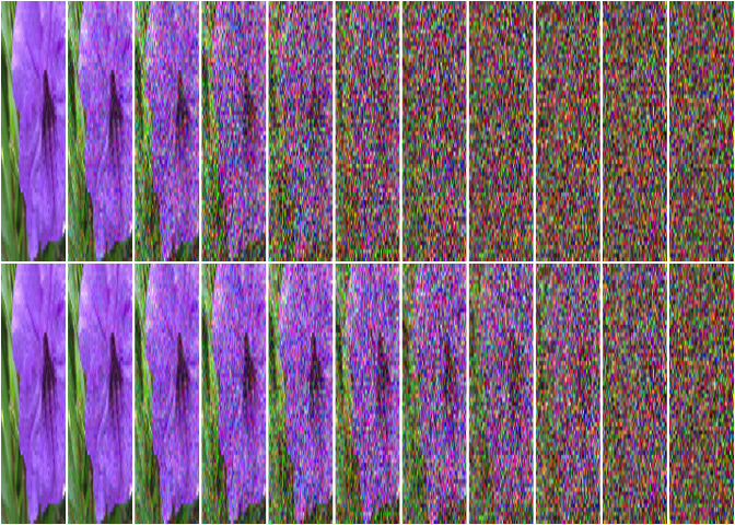
Model trained, the reverse process – image generation – is straightforward: It consists in recursive de-noising according to the (known) noise rate schedule. All in all, the complete process then might look like this:
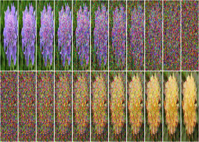
Wrapping up, this post, by itself, is really just an invitation. To find out more, check out the GitHub repository. Should you need additional motivation to do so, here are some flower images.

Thanks for reading!